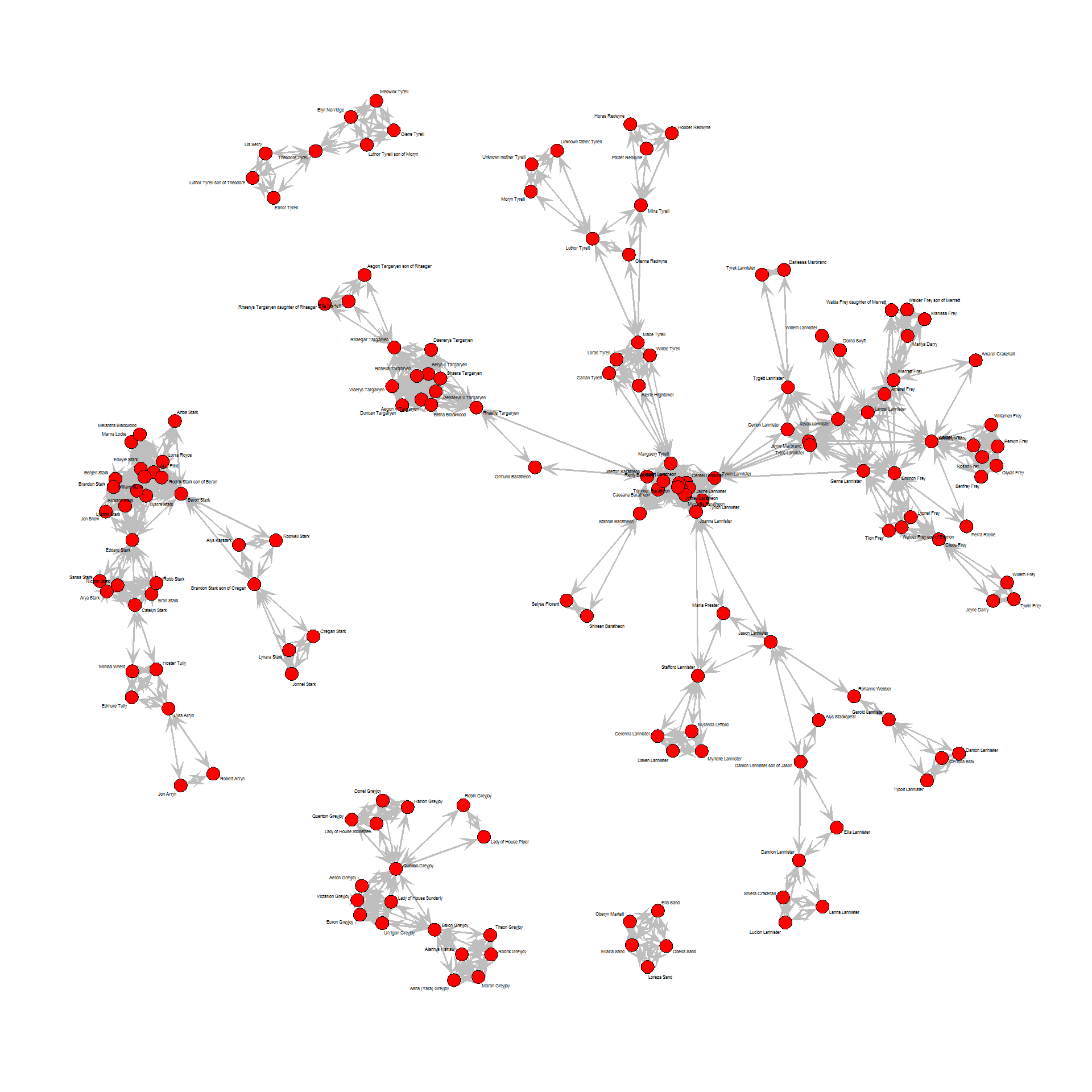
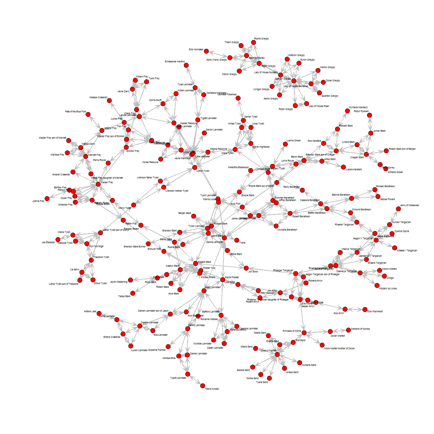
In this post, I am exploring network analysis techniques in a family network of major characters from Game of Thrones.
Not surprisingly, we learn that House Stark (specifically Ned and Sansa) and House Lannister (especially Tyrion) are the most important family connections in Game of Thrones; they also connect many of the storylines and are central parts of the narrative.
What is a network?
A network in this context is a graph of interconnected nodes/vertices. Nodes can e.g. be people in a social network, genes in a co-expression network, etc. Nodes are connected via ties/edges.
What can network analysis tell us?
Network analysis can e.g. be used to explore relationships in social or professional networks. In such cases, we would typically ask questions like:
- How many connections does each person have?
- Who is the most connected (i.e. influential or “important”) person?
- Are there clusters of tightly connected people?
- Are there a few key players that connect clusters of people?
- etc.
These answers can give us a lot of information about the patterns of how people interact.
The Game of Thrones character network
The basis for this network is Kaggle’s Game of Throne dataset (character-deaths.csv). Because most family relationships were missing in that dataset, I added the missing information in part by hand (based on A Wiki of Ice and Fire) and by scraping information from the Game of Thrones wiki. You can find the full code for how I generated the network on my Github page.
library(tidyverse)
library(igraph)
library(statnet)
load("union_edges.RData")
load("union_characters.RData")
I am using igraph to plot the initial network. To do so, I first create the graph from the edge- and node-table. An edge-table contains source and target nodes in the first two columns and optionally additional columns with edge attributes. Here, I have the type of interaction (mother, father or spouse), the color and line-type I want to assign to each edge.
Because the books and the TV series differ slightly, I have introduced edges that are only supported or hinted at by the TV series and are not part of the original narrative in the books. These edges are marked by being dotted instead of solid. An additional color for edges with unspecified parental origin are introduced as well. Originally, these served for interactions that were extracted from character names (i.e. characters that ended with “… son/daughter of …”) and could either mean mother or father. Now, they show unclear parentage or cases where there are a biological and a de facto father, as in the case of Jon Snow.
head(union_edges)
##               source            target   type   color   lty
## 1         Lysa Arryn      Robert Arryn mother #7570B3 solid
## 2       Jasper Arryn        Alys Arryn father #1B9E77 solid
## 3       Jasper Arryn         Jon Arryn father #1B9E77 solid
## 4          Jon Arryn      Robert Arryn father #1B9E77 solid
## 110 Cersei Lannister  Tommen Baratheon mother #7570B3 solid
## 210 Cersei Lannister Joffrey Baratheon mother #7570B3 solid
The nodetable contains one row for each character that is either a source or a target in the edgetable. We can give any number and type of node attributes. Here, I chose the followin columns from the original Kaggle dataset: gender/male (male = 1, female = 0), house (as the house each character was born into) and popularity. House2 was meant to assign a color to only the major houses. Shape represents the gender.
head(union_characters)
##            name male culture          house popularity      house2   color  shape
## 1    Alys Arryn    0    <NA>    House Arryn 0.08026756        <NA>    <NA> circle
## 2 Elys Waynwood    0    <NA> House Waynwood 0.07023411        <NA>    <NA> circle
## 3  Jasper Arryn    1    <NA>    House Arryn 0.04347826        <NA>    <NA> square
## 4   Jeyne Royce    0    <NA>    House Royce 0.00000000        <NA>    <NA> circle
## 5     Jon Arryn    1 Valemen    House Arryn 0.83612040        <NA>    <NA> square
## 6    Lysa Arryn    0    <NA>    House Tully 0.00000000 House Tully #F781BF circle
By default, we have a directed graph.
union_graph <- graph_from_data_frame(union_edges, directed = TRUE, vertices = union_characters)
For plotting the legend, I am summarizing the edge and node colors.
color_vertices <- union_characters %>%
  group_by(house, color) %>%
  summarise(n = n()) %>%
  filter(!is.na(color))

colors_edges <- union_edges %>%
  group_by(type, color) %>%
  summarise(n = n()) %>%
  filter(!is.na(color))
Now, we can plot the graph object (here with Fruchterman-Reingold layout):
layout <- layout_with_fr(union_graph)
Click on the image to get to the high resolution pdf:
plot(union_graph,
     layout = layout,
     vertex.label = gsub(" ", "\n", V(union_graph)$name),
     vertex.shape = V(union_graph)$shape,
     vertex.color = V(union_graph)$color,
     vertex.size = (V(union_graph)$popularity + 0.5) * 5,
     vertex.frame.color = "gray",
     vertex.label.color = "black",
     vertex.label.cex = 0.8,
     edge.arrow.size = 0.5,
     edge.color = E(union_graph)$color,
     edge.lty = E(union_graph)$lty)
legend("topleft", legend = c(NA, "Node color:", as.character(color_vertices$house), NA, "Edge color:", as.character(colors_edges$type)), pch = 19,
       col = c(NA, NA, color_vertices$color, NA, NA, colors_edges$color), pt.cex = 5, cex = 2, bty = "n", ncol = 1,
       title = "")
legend("topleft", legend = "", cex = 4, bty = "n", ncol = 1,
       title = "Game of Thrones Family Ties")
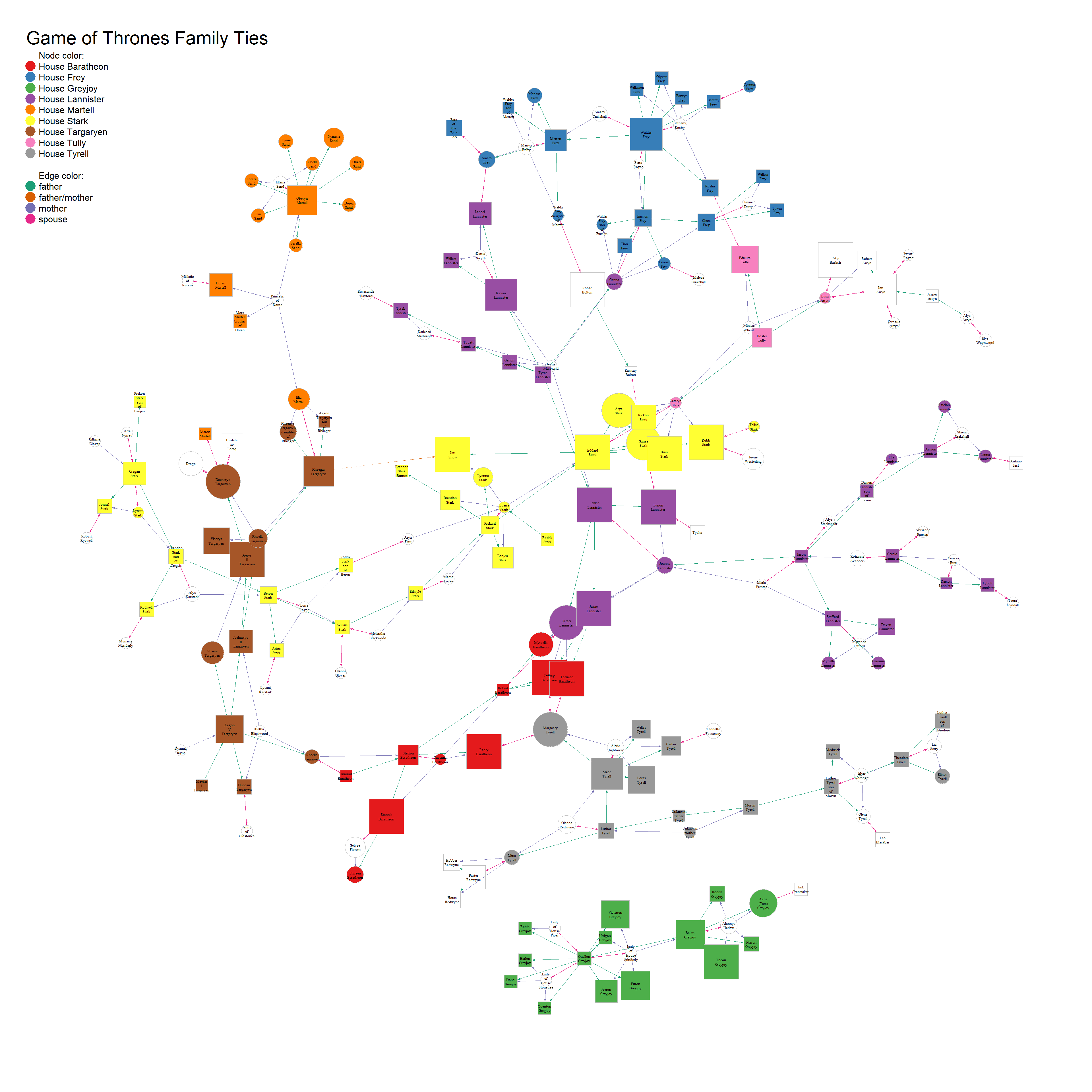
Node color shows the major houses, node size the character’s popularity and node shape their gender (square for male, circle for female). Edge color shows interaction type.
As we can see, even with only a subset of characters from the Game of Thrones world, the network is already quite big. You can click on the image to open the pdf and zoom into specific parts of the plot and read the node labels/character names.
What we can see right away is that there are only limited connections between houses and that the Greyjoys are the only house that has no ties to any of the others.
Network analysis
How do we find out who the most important characters are in this network?
We consider a character “important” if he has connections to many other characters. There are a few network properties, that tell us more about this. For this, I am considering the network as undirected to account for parent/child relationships as being mutual.
union_graph_undir <- as.undirected(union_graph, mode = "collapse")
Centrality
Centrality describes the number of edges that are in- or outgoing to/from nodes. High centrality networks have few nodes with many connections, low centrality networks have many nodes with similar numbers of edges.
“Centralization is a method for creating a graph level centralization measure from the centrality scores of the vertices.” centralize() help
For the whole network, we can calculate centrality by degree (centr_degree()), closeness (centr_clo()) or eigenvector centrality (centr_eigen()) of vertices.
centr_degree(union_graph_undir, mode = "total")$centralization
## [1] 0.04282795
centr_clo(union_graph_undir, mode = "total")$centralization
## [1] 0.01414082
centr_eigen(union_graph_undir, directed = FALSE)$centralization
## [1] 0.8787532
Node degree
Node degree or degree centrality describes how central a node is in the network (i.e. how many in- and outgoing edges it has or to how many other nodes it is directly connected via one edge).
“The degree of a vertex is its most basic structural property, the number of its adjacent edges.” From the help pages of degree()
We can calculate the number of out- or ingoing edges of each node, or - as I am doing here - the sum of both.
union_graph_undir_degree <- igraph::degree(union_graph_undir, mode = "total")

#standardized by number of nodes
union_graph_undir_degree_std <- union_graph_undir_degree / (vcount(union_graph_undir) - 1)
node_degree <- data.frame(degree = union_graph_undir_degree,
                          degree_std = union_graph_undir_degree_std) %>%
  tibble::rownames_to_column()

union_characters <- left_join(union_characters, node_degree, by = c("name" = "rowname"))

node_degree %>%
  arrange(-degree) %>%
  .[1:10, ]
##            rowname degree degree_std
## 1  Quellon Greyjoy     12 0.05797101
## 2      Walder Frey     10 0.04830918
## 3   Oberyn Martell     10 0.04830918
## 4     Eddard Stark      9 0.04347826
## 5    Catelyn Stark      8 0.03864734
## 6       Emmon Frey      7 0.03381643
## 7  Genna Lannister      7 0.03381643
## 8     Merrett Frey      7 0.03381643
## 9    Balon Greyjoy      7 0.03381643
## 10 Jason Lannister      7 0.03381643
In this case, the node degree reflects how many offspring and spouses a character had. With 3 wifes and several children, Quellon Greyjoy, the grandfather of Theon and Asha/Yara comes out on top (of course, had I included all offspring and wifes of Walder Frey’s, he would easily be on top but the network would have gotten infinitely more confusing).
Closeness
The closeness of a node describes its distance to all other nodes. A node with highest closeness is more central and can spread information to many other nodes.
closeness <- igraph::closeness(union_graph_undir, mode = "total")

#standardized by number of nodes
closeness_std <- closeness / (vcount(union_graph_undir) - 1)
node_closeness <- data.frame(closeness = closeness,
                          closeness_std = closeness_std) %>%
  tibble::rownames_to_column()

union_characters <- left_join(union_characters, node_closeness, by = c("name" = "rowname"))

node_closeness %>%
  arrange(-closeness) %>%
  .[1:10, ]
##             rowname    closeness closeness_std
## 1       Sansa Stark 0.0002013288  9.726028e-07
## 2  Tyrion Lannister 0.0002012882  9.724070e-07
## 3   Tywin Lannister 0.0002011668  9.718201e-07
## 4  Joanna Lannister 0.0002005616  9.688965e-07
## 5      Eddard Stark 0.0002002804  9.675381e-07
## 6     Catelyn Stark 0.0001986492  9.596579e-07
## 7  Cersei Lannister 0.0001984915  9.588960e-07
## 8   Jaime Lannister 0.0001975894  9.545382e-07
## 9    Jeyne Marbrand 0.0001966568  9.500330e-07
## 10  Tytos Lannister 0.0001966568  9.500330e-07
The characters with highest closeness all surround central characters that connect various storylines and houses in Game of Thrones.
Betweenness centrality
Betweenness describes the number of shortest paths between nodes. Nodes with high betweenness centrality are on the path between many other nodes, i.e. they are people who are key connections or bridges between different groups of nodes. In a social network, these nodes would be very important because they are likely to pass on information to a wide reach of people.
The igraph function betweenness() calculates vertex betweenness, edge_betweenness() calculates edge betweenness:
“The vertex and edge betweenness are (roughly) defined by the number of geodesics (shortest paths) going through a vertex or an edge.” igraph help for estimate_betweenness()
betweenness <- igraph::betweenness(union_graph_undir, directed = FALSE)

# standardize by number of node pairs
betweenness_std <- betweenness / ((vcount(union_graph_undir) - 1) * (vcount(union_graph_undir) - 2) / 2)

node_betweenness <- data.frame(betweenness = betweenness,
                               betweenness_std = betweenness_std) %>%
  tibble::rownames_to_column()

union_characters <- left_join(union_characters, node_betweenness, by = c("name" = "rowname"))

node_betweenness %>%
  arrange(-betweenness) %>%
  .[1:10, ]
##              rowname betweenness betweenness_std
## 1       Eddard Stark    6926.864       0.3248846
## 2        Sansa Stark    6165.667       0.2891828
## 3   Tyrion Lannister    5617.482       0.2634718
## 4    Tywin Lannister    5070.395       0.2378123
## 5   Joanna Lannister    4737.524       0.2221999
## 6  Rhaegar Targaryen    4301.583       0.2017533
## 7    Margaery Tyrell    4016.417       0.1883784
## 8           Jon Snow    3558.884       0.1669192
## 9        Mace Tyrell    3392.500       0.1591154
## 10   Jason Lannister    3068.500       0.1439191
edge_betweenness <- igraph::edge_betweenness(union_graph_undir, directed = FALSE)

data.frame(edge = attr(E(union_graph_undir), "vnames"),
           betweenness = edge_betweenness) %>%
  tibble::rownames_to_column() %>%
  arrange(-betweenness) %>%
  .[1:10, ]
##    rowname                              edge betweenness
## 1      160      Sansa Stark|Tyrion Lannister    5604.149
## 2      207          Sansa Stark|Eddard Stark    4709.852
## 3      212        Rhaegar Targaryen|Jon Snow    3560.083
## 4      296       Margaery Tyrell|Mace Tyrell    3465.000
## 5      213             Eddard Stark|Jon Snow    3163.048
## 6      131  Jason Lannister|Joanna Lannister    3089.500
## 7      159 Joanna Lannister|Tyrion Lannister    2983.591
## 8      171  Tyrion Lannister|Tywin Lannister    2647.224
## 9      192    Elia Martell|Rhaegar Targaryen    2580.000
## 10     300         Luthor Tyrell|Mace Tyrell    2565.000
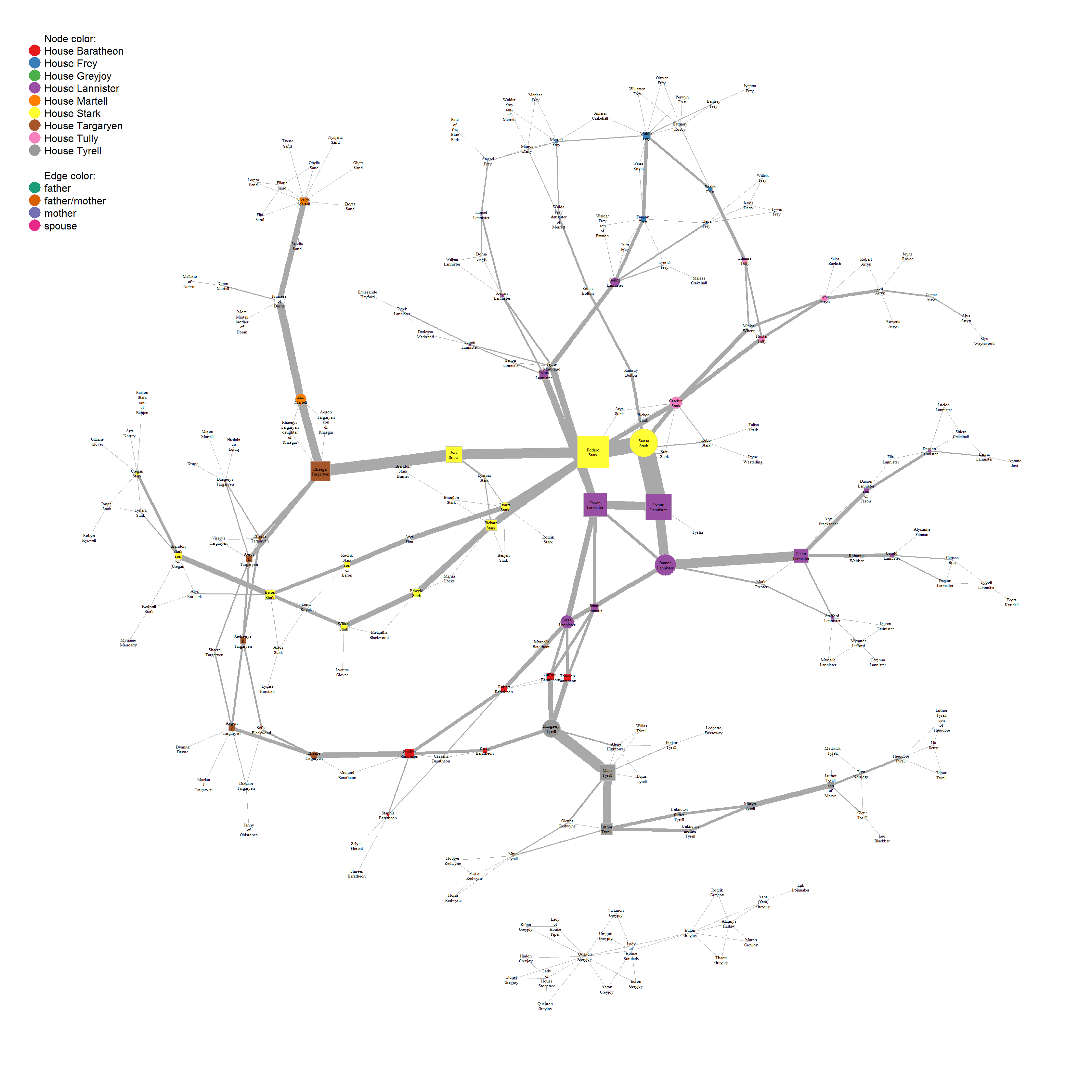
This, we can now plot by feeding the node betweenness as vertex.size and edge betweenness as edge.width to our plot function:
plot(union_graph_undir,
     layout = layout,
     vertex.label = gsub(" ", "\n", V(union_graph_undir)$name),
     vertex.shape = V(union_graph_undir)$shape,
     vertex.color = V(union_graph_undir)$color,
     vertex.size = betweenness * 0.001,
     vertex.frame.color = "gray",
     vertex.label.color = "black",
     vertex.label.cex = 0.8,
     edge.width = edge_betweenness * 0.01,
     edge.arrow.size = 0.5,
     edge.color = E(union_graph_undir)$color,
     edge.lty = E(union_graph_undir)$lty)
legend("topleft", legend = c("Node color:", as.character(color_vertices$house), NA, "Edge color:", as.character(colors_edges$type)), pch = 19,
       col = c(NA, color_vertices$color, NA, NA, colors_edges$color), pt.cex = 5, cex = 2, bty = "n", ncol = 1)
Ned Stark is the character with highest betweenness. This makes sense, as he and his children (specifically Sansa and her arranged marriage to Tyrion) connect to other houses and are the central points from which the story unfolds. However, we have to keep in mind here, that my choice of who is important enough to include in the network (e.g. the Stark ancestors) and who not (e.g. the whole complicated mess that is the Targaryen and Frey family tree) makes this result somewhat biased.
Diameter
In contrast to the shortest path between two nodes, we can also calculate the longest path, or diameter:
diameter(union_graph_undir, directed = FALSE)
## [1] 21
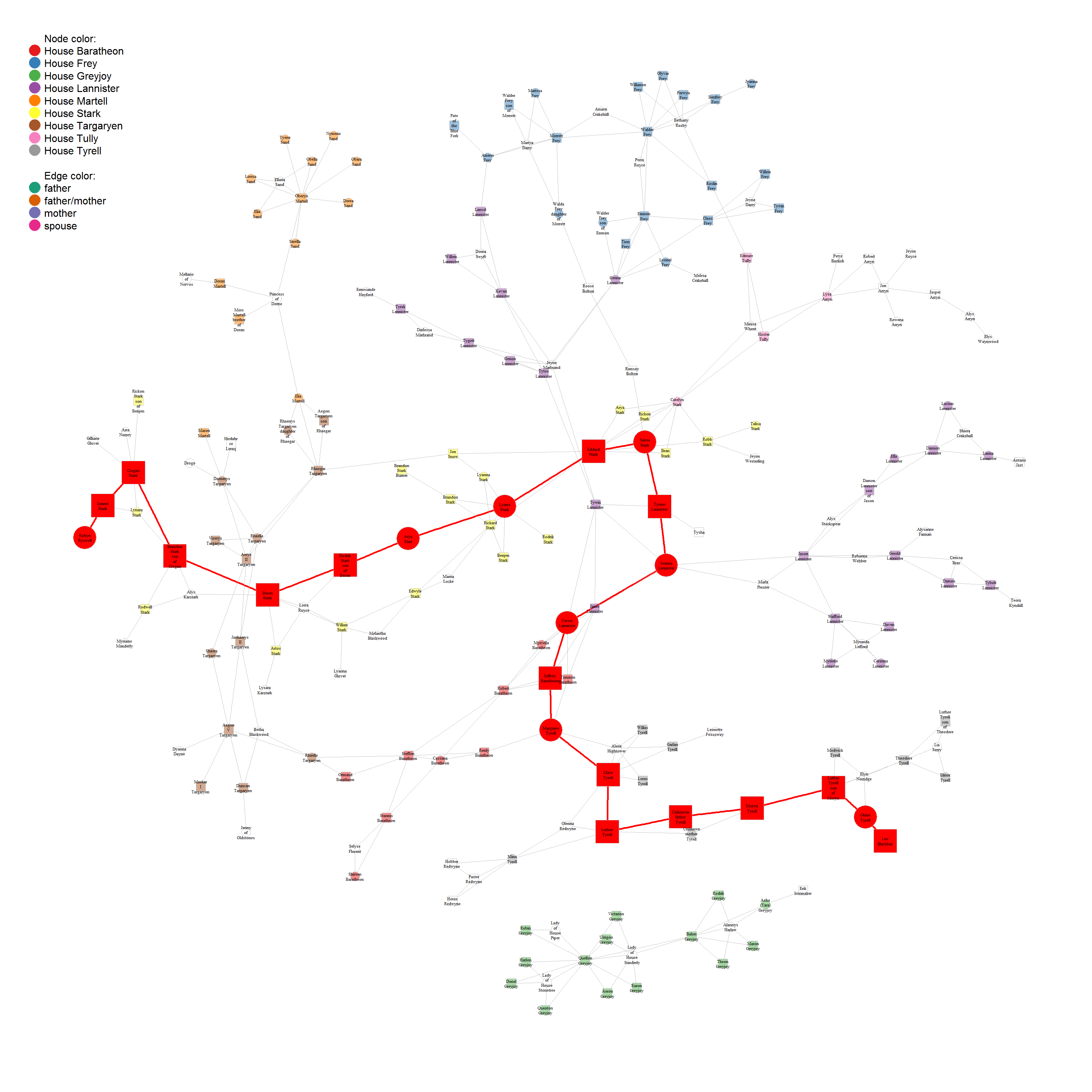
In our network, the longest path connects 21 nodes.
“get_diameter returns a path with the actual diameter. If there are many shortest paths of the length of the diameter, then it returns the first one found.” diameter() help
This, we can also plot:
union_graph_undir_diameter <- union_graph_undir
node_diameter <- get.diameter(union_graph_undir_diameter,  directed = FALSE)

V(union_graph_undir_diameter)$color <- scales::alpha(V(union_graph_undir_diameter)$color, alpha = 0.5)
V(union_graph_undir_diameter)$size <- 2

V(union_graph_undir_diameter)[node_diameter]$color <- "red"
V(union_graph_undir_diameter)[node_diameter]$size <- 5

E(union_graph_undir_diameter)$color <- "grey"
E(union_graph_undir_diameter)$width <- 1

E(union_graph_undir_diameter, path = node_diameter)$color <- "red"
E(union_graph_undir_diameter, path = node_diameter)$width <- 5

plot(union_graph_undir_diameter,
     layout = layout,
     vertex.label = gsub(" ", "\n", V(union_graph_undir_diameter)$name),
     vertex.shape = V(union_graph_undir_diameter)$shape,
     vertex.frame.color = "gray",
     vertex.label.color = "black",
     vertex.label.cex = 0.8,
     edge.arrow.size = 0.5,
     edge.lty = E(union_graph_undir_diameter)$lty)
legend("topleft", legend = c("Node color:", as.character(color_vertices$house), NA, "Edge color:", as.character(colors_edges$type)), pch = 19,
       col = c(NA, color_vertices$color, NA, NA, colors_edges$color), pt.cex = 5, cex = 2, bty = "n", ncol = 1)
Transitivity
“Transitivity measures the probability that the adjacent vertices of a vertex are connected. This is sometimes also called the clustering coefficient.” transitivity() help
We can calculate the transitivity or ratio of triangles to connected triples for the whole network:
transitivity(union_graph_undir, type = "global")
## [1] 0.2850679
Or for each node:
transitivity <- data.frame(name = V(union_graph_undir)$name,
      transitivity = transitivity(union_graph_undir, type = "local")) %>%
  mutate(name = as.character(name))

union_characters <- left_join(union_characters, transitivity, by = "name")

transitivity %>%
  arrange(-transitivity) %>%
  .[1:10, ]
##                 name transitivity
## 1       Robert Arryn            1
## 2   Ormund Baratheon            1
## 3     Selyse Florent            1
## 4  Shireen Baratheon            1
## 5   Amarei Crakehall            1
## 6       Marissa Frey            1
## 7        Olyvar Frey            1
## 8        Perra Royce            1
## 9        Perwyn Frey            1
## 10         Tion Frey            1
Because ours is a family network, characters with a transitivity of one form triangles with their parents or offspring.
PageRank centrality
PageRank (originally used by Google to rank the importance of search results) is similar to eigenvector centrality. Eigenvector centrality scores nodes in a network according to the number of connections to high-degree nodes they have. It is therefore a measure of node importance. PageRank similarly considers nodes as more important if they have many incoming edges (or links).
page_rank <- page.rank(union_graph_undir, directed = FALSE)

page_rank_centrality <- data.frame(name = names(page_rank$vector),
      page_rank = page_rank$vector) %>%
  mutate(name = as.character(name))

union_characters <- left_join(union_characters, page_rank_centrality, by = "name")

page_rank_centrality %>%
  arrange(-page_rank) %>%
  .[1:10, ]
##                 name   page_rank
## 1     Oberyn Martell 0.018402407
## 2    Quellon Greyjoy 0.016128129
## 3        Walder Frey 0.012956029
## 4       Eddard Stark 0.011725019
## 5       Cregan Stark 0.010983561
## 6      Catelyn Stark 0.010555473
## 7       Lyarra Stark 0.009876629
## 8  Aegon V Targaryen 0.009688458
## 9      Balon Greyjoy 0.009647049
## 10         Jon Arryn 0.009623742
Oberyn Martell, Quellon Greyjoy and Walder Frey all have the highest number of spouses, children and grandchildren are are therefore scored highest for PageRank.
Matrix representation of a network
Connections between nodes can also be represented as an adjacency matrix. We can convert our graph object to an adjacency matrix with igraph’s as_adjacency_matrix() function. Whenever there is an edge between two nodes, this field in the matrix will get assigned a 1, otherwise it is 0.
adjacency <- as.matrix(as_adjacency_matrix(union_graph_undir))
Eigenvector centrality
We can now calculate the eigenvalues and eigenvectors of the adjacency matrix.
#degree diagonal matrix
degree_diag <- diag(1 / igraph::degree(union_graph_undir))

# PageRank matrix
pagerank <- adjacency %*% degree_diag

eigenvalues <- eigen(pagerank)
The eigenvector with the highest eigenvalue scores those vertices highly, that have many eges or that are connected to vertices with many edges.
eigenvector <- data.frame(name = rownames(pagerank),
           eigenvector = as.numeric(eigenvalues$vectors[, which.max(eigenvalues$values)]))

union_characters <- left_join(union_characters, eigenvector, by = "name")

eigenvector %>%
  arrange(eigenvector) %>%
  .[1:10, ]
##                       name eigenvector
## 1          Quellon Greyjoy  -0.6625628
## 2            Balon Greyjoy  -0.3864950
## 3   Lady of House Sunderly  -0.3312814
## 4           Alannys Harlaw  -0.2760678
## 5  Lady of House Stonetree  -0.2208543
## 6      Asha (Yara) Greyjoy  -0.1656407
## 7            Robin Greyjoy  -0.1104271
## 8            Euron Greyjoy  -0.1104271
## 9          Urrigon Greyjoy  -0.1104271
## 10       Victarion Greyjoy  -0.1104271
Because of their highly connected family ties (i.e. there are only a handful of connections but they are almost all triangles), the Greyjoys have been scored with the highest eigenvalues.
We can find the eigenvector centrality scores with:
eigen_centrality <- igraph::eigen_centrality(union_graph_undir, directed = FALSE)

eigen_centrality <- data.frame(name = names(eigen_centrality$vector),
           eigen_centrality = eigen_centrality$vector) %>%
  mutate(name = as.character(name))

union_characters <- left_join(union_characters, eigen_centrality, eigenvector, by = "name")

eigen_centrality %>%
  arrange(-eigen_centrality) %>%
  .[1:10, ]
##                name eigen_centrality
## 1   Tywin Lannister        1.0000000
## 2  Cersei Lannister        0.9168980
## 3  Joanna Lannister        0.8358122
## 4    Jeyne Marbrand        0.8190076
## 5   Tytos Lannister        0.8190076
## 6   Genna Lannister        0.7788376
## 7   Jaime Lannister        0.7642870
## 8  Robert Baratheon        0.7087042
## 9        Emmon Frey        0.6538709
## 10      Walder Frey        0.6516021
When we consider eigenvector centrality, Tywin and the core Lannister family score highest.
Who are the most important characters?
We can now compare all the node-level information to decide which characters are the most important in Game of Thrones. Such node level characteristics could also be used as input for machine learning algorithms.
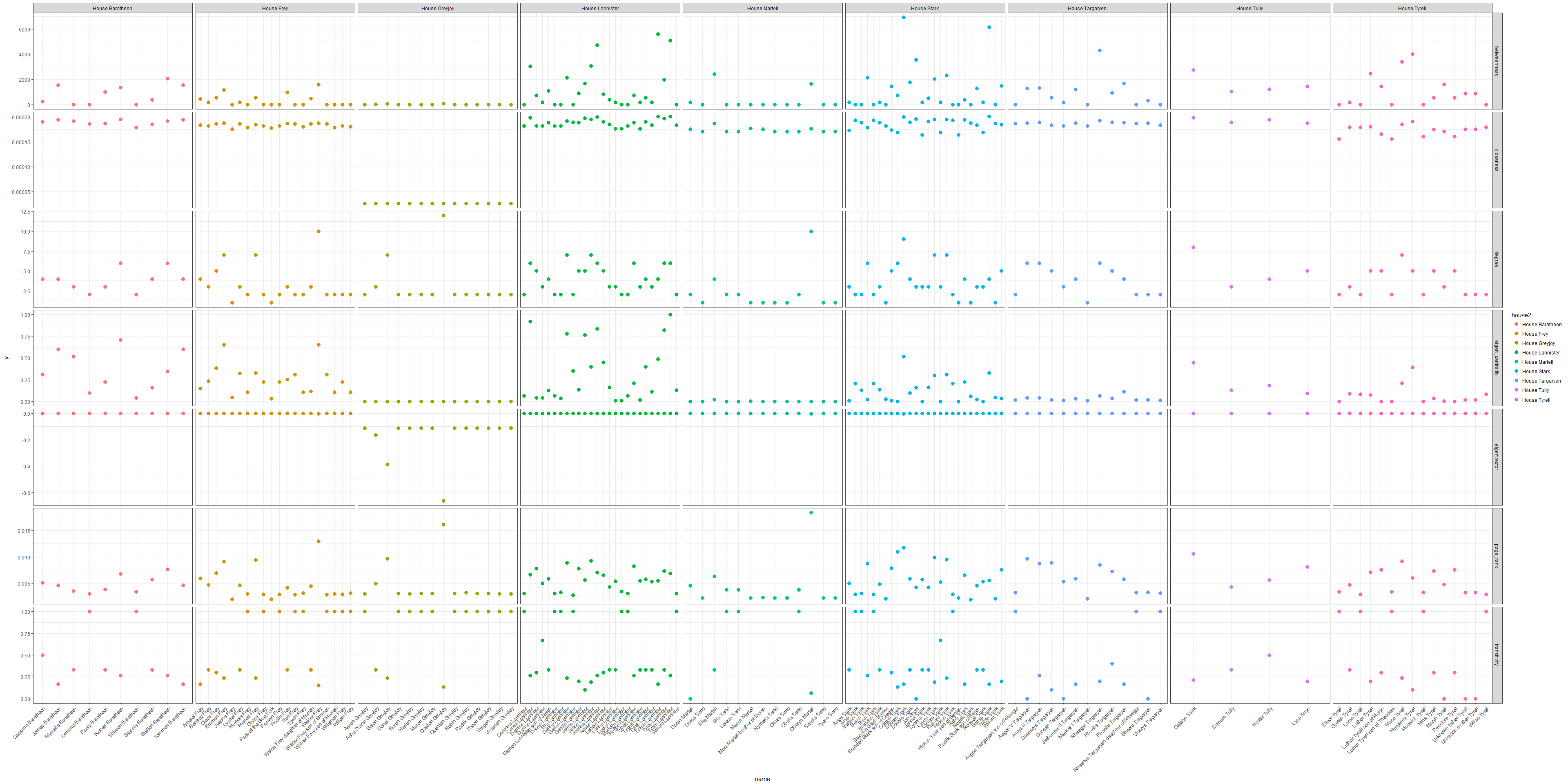
Let’s look at all characters from the major houses:
union_characters %>%
  filter(!is.na(house2)) %>%
  dplyr::select(-contains("_std")) %>%
  gather(x, y, degree:eigen_centrality) %>%
  ggplot(aes(x = name, y = y, color = house2)) +
    geom_point(size = 3) +
    facet_grid(x ~ house2, scales = "free") +
    theme_bw() +
    theme(axis.text.x = element_text(angle = 45, vjust = 1, hjust=1))
Taken together, we could say that House Stark (specifically Ned and Sansa) and House Lannister (especially Tyrion) are the most important family connections in Game of Thrones.
Groups of nodes
We can also analyze dyads (pairs of two nodes), triads (groups of three nodes) and bigger cliques in our network. For dyads, we can use the function dyad_census() from igraph or dyad.census() from sna. Both are identical and calculate a Holland and Leinhardt dyad census with
- mut: The number of pairs with mutual connections (in our case, spouses).
- asym: The number of pairs with non-mutual connections (in the original network: mother-child and father-child relationships; but in the undirected network, there are none).
- null: The number of pairs with no connection between them.
#igraph::dyad_census(union_graph_undir)
sna::dyad.census(adjacency)
##      Mut Asym  Null
## [1,] 326    0 21202
The same can be calculated for triads (see ?triad_census for details on what each output means).
#igraph::triad_census(union_graph_undir)
sna::triad.census(adjacency)
##          003 012   102 021D 021U 021C 111D 111U 030T 030C 201 120D 120U 120C 210 300
## [1,] 1412100   0 65261    0    0    0    0    0    0    0 790    0    0    0   0 105
triad.classify(adjacency, mode = "graph")
## [1] 2
We can also calculate the number of paths and cycles of any length we specify, here e.g. of length <= 5. For edges, we obtain the sum of counts for all paths or cycles up to the given maximum length. For vertices/nodes, we obtain the number of paths or cycles to which each node belongs.
node_kpath <- kpath.census(adjacency, maxlen = 5, mode = "graph", tabulate.by.vertex = TRUE, dyadic.tabulation = "sum")
edge_kpath <- kpath.census(adjacency, maxlen = 5, mode = "graph", tabulate.by.vertex = FALSE)
edge_kpath
## $path.count
##     1     2     3     4     5
##   326  1105  2973  7183 17026
This, we could plot with (but here, it does not give much additional information):
gplot(node_kpath$paths.bydyad,
      label.cex = 0.5,
      vertex.cex = 0.75,
      displaylabels = TRUE,
      edge.col = "grey")
node_kcycle <- kcycle.census(adjacency, maxlen = 8, mode = "graph", tabulate.by.vertex = TRUE, cycle.comembership = "sum")
edge_kcycle <- kcycle.census(adjacency, maxlen = 8, mode = "graph", tabulate.by.vertex = FALSE)
edge_kcycle
## $cycle.count
##   2   3   4   5   6   7   8
##   0 105 136  27  57  58  86
node_kcycle_reduced <- node_kcycle$cycle.comemb
node_kcycle_reduced <- node_kcycle_reduced[which(rowSums(node_kcycle_reduced) > 0), which(colSums(node_kcycle_reduced) > 0)]

gplot(node_kcycle_reduced,
      label.cex = 0.5,
      vertex.cex = 0.75,
      displaylabels = TRUE,
      edge.col = "grey")
“A (maximal) clique is a maximal set of mutually adjacency vertices.” clique.census() help
node_clique <- clique.census(adjacency, mode = "graph", tabulate.by.vertex = TRUE, clique.comembership = "sum")
edge_clique <- clique.census(adjacency, mode = "graph", tabulate.by.vertex = FALSE, clique.comembership = "sum")
edge_clique$clique.count
##   1   2   3
##   0  74 105
node_clique_reduced <- node_clique$clique.comemb
node_clique_reduced <- node_clique_reduced[which(rowSums(node_clique_reduced) > 0), which(colSums(node_clique_reduced) > 0)]

gplot(node_clique_reduced,
      label.cex = 0.5,
      vertex.cex = 0.75,
      displaylabels = TRUE,
      edge.col = "grey")
The largest group of nodes ín this network is three, i.e. all parent/child relationships. Therefore, it does not really make sense to plot them all, but we could plot and color them with:
vcol <- rep("grey80", vcount(union_graph_undir))

# highlight first of largest cliques
vcol[unlist(largest_cliques(union_graph_undir)[[1]])] <- "red"

plot(union_graph_undir,
     layout = layout,
     vertex.label = gsub(" ", "\n", V(union_graph_undir)$name),
     vertex.shape = V(union_graph_undir)$shape,
     vertex.color = vcol,
     vertex.size = 5,
     vertex.frame.color = "gray",
     vertex.label.color = "black",
     vertex.label.cex = 0.8,
     edge.width = 2,
     edge.arrow.size = 0.5,
     edge.color = E(union_graph_undir)$color,
     edge.lty = E(union_graph_undir)$lty)
Clustering
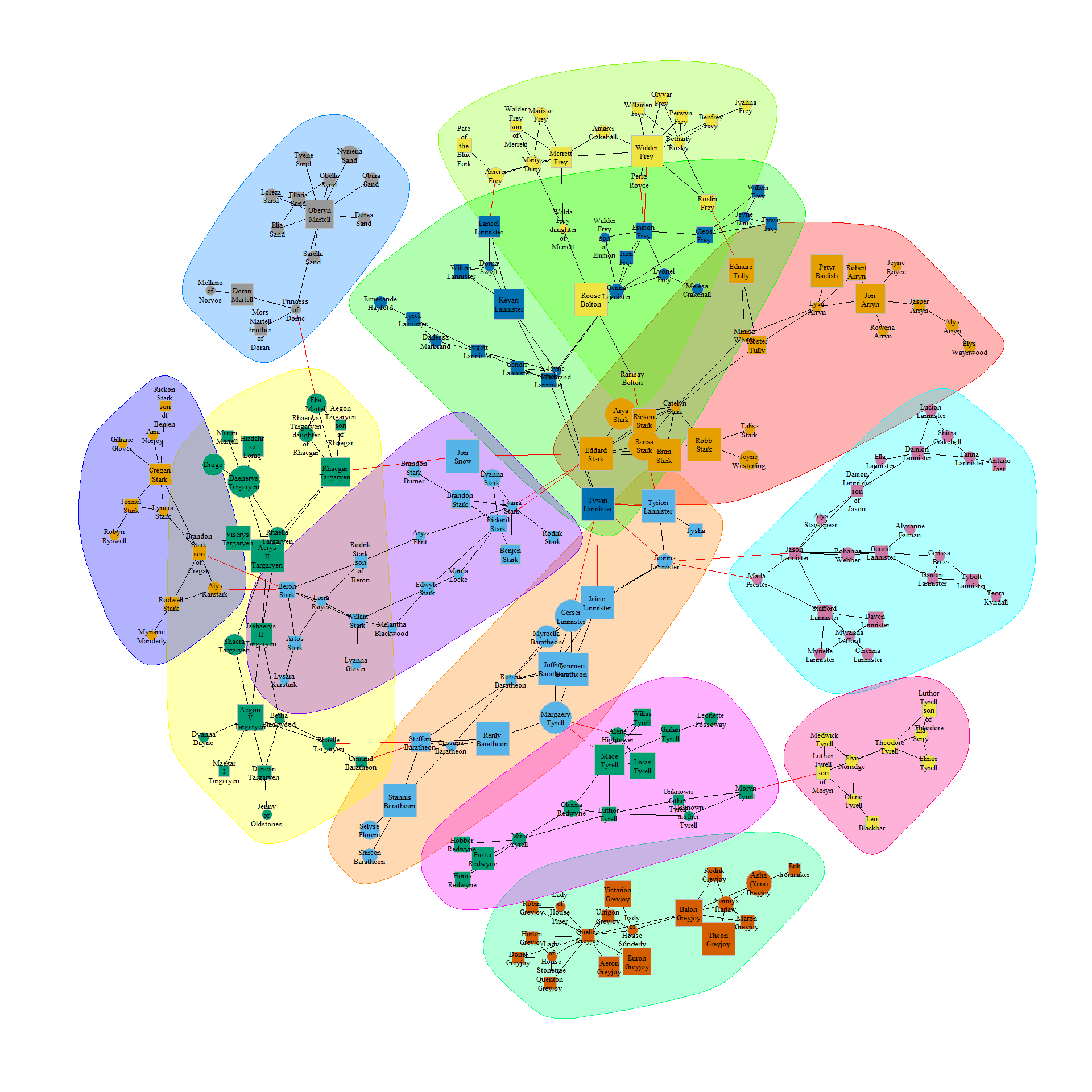
We can also look for groups within our network by clustering node groups according to their edge betweenness:
ceb <- cluster_edge_betweenness(union_graph_undir)
modularity(ceb)
## [1] 0.8359884
plot(ceb,
     union_graph_undir,
     layout = layout,
     vertex.label = gsub(" ", "\n", V(union_graph_undir)$name),
     vertex.shape = V(union_graph_undir)$shape,
     vertex.size = (V(union_graph_undir)$popularity + 0.5) * 5,
     vertex.frame.color = "gray",
     vertex.label.color = "black",
     vertex.label.cex = 0.8)
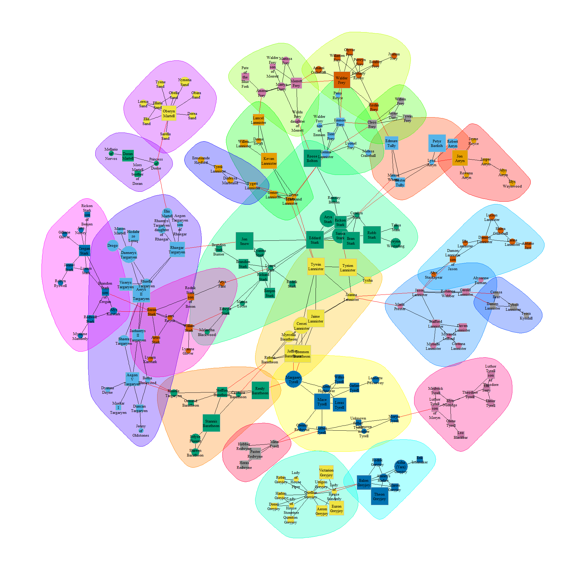
Or based on propagating labels:
clp <- cluster_label_prop(union_graph_undir)

plot(clp,
     union_graph_undir,
     layout = layout,
     vertex.label = gsub(" ", "\n", V(union_graph_undir)$name),
     vertex.shape = V(union_graph_undir)$shape,
     vertex.size = (V(union_graph_undir)$popularity + 0.5) * 5,
     vertex.frame.color = "gray",
     vertex.label.color = "black",
     vertex.label.cex = 0.8)
Network properties
We can also feed our adjacency matrix to other functions, like GenInd() from the NetIndices packages. This function calculates a number of network properties, like number of compartments (N), total system throughput (T..), total system throughflow (TST), number of internal links (Lint), total number of links (Ltot), like density (LD), connectance (C), average link weight (Tijbar), average compartment throughflow (TSTbar) and compartmentalization or degree of connectedness of subsystems in the network (Cbar).
library(NetIndices)
graph.properties <- GenInd(adjacency)
graph.properties
## $N
## [1] 208
##
## $T..
## [1] 652
##
## $TST
## [1] 652
##
## $Lint
## [1] 652
##
## $Ltot
## [1] 652
##
## $LD
## [1] 3.134615
##
## $C
## [1] 0.01514307
##
## $Tijbar
## [1] 1
##
## $TSTbar
## [1] 3.134615
##
## $Cbar
## [1] 0.01086163
Alternatively, the network package provides additional functions to obtain network properties. Here, we can again feed in the adjacency matrix of our network and convert it to a network object.
library(network)
adj_network <- network(adjacency, directed = TRUE)
adj_network
##  Network attributes:
##   vertices = 208
##   directed = TRUE
##   hyper = FALSE
##   loops = FALSE
##   multiple = FALSE
##   bipartite = FALSE
##   total edges= 652
##     missing edges= 0
##     non-missing edges= 652
##
##  Vertex attribute names:
##     vertex.names
##
## No edge attributes
From this network object, we can e.g. get the number of dyads and edges within a network and the network size.
network.dyadcount(adj_network)
## [1] 43056
network.edgecount(adj_network)
## [1] 652
network.size(adj_network)
## [1] 208
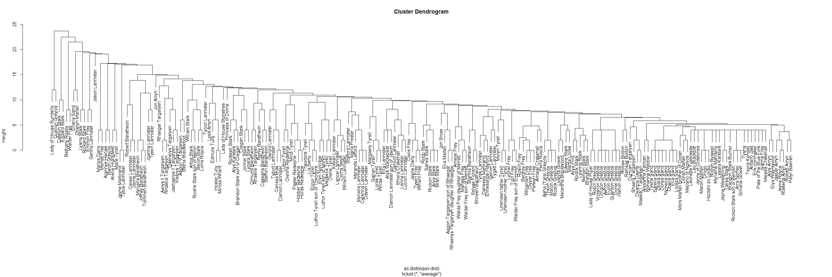
“equiv.clust uses a definition of approximate equivalence (equiv.fun) to form a hierarchical clustering of network positions. Where dat consists of multiple relations, all specified relations are considered jointly in forming the equivalence clustering.” equiv.clust() help
ec <- equiv.clust(adj_network, mode = "graph", cluster.method = "average", plabels = network.vertex.names(adj_network))
ec
## Position Clustering:
##
##  Equivalence function: sedist
##  Equivalence metric: hamming
##  Cluster method: average
##  Graph order: 208
ec$cluster$labels <- ec$plabels
plot(ec)
From the sna package, we can e.g. use functions that tell us the graph density and the dyadic reciprocity of the vertices or edges
gden(adjacency)
## [1] 0.01514307
grecip(adjacency)
## Mut
##   1
grecip(adjacency, measure = "edgewise")
## Mut
##   1
sessionInfo()
## R version 3.4.0 (2017-04-21)
## Platform: x86_64-w64-mingw32/x64 (64-bit)
## Running under: Windows 7 x64 (build 7601) Service Pack 1
##
## Matrix products: default
##
## locale:
## [1] LC_COLLATE=English_United States.1252  LC_CTYPE=English_United States.1252    LC_MONETARY=English_United States.1252 LC_NUMERIC=C                           LC_TIME=English_United States.1252
##
## attached base packages:
## [1] stats     graphics  grDevices utils     datasets  methods   base
##
## other attached packages:
##  [1] NetIndices_1.4.4     MASS_7.3-47          statnet_2016.9       sna_2.4              ergm.count_3.2.2     tergm_3.4.0          networkDynamic_0.9.0 ergm_3.7.1           network_1.13.0       statnet.common_3.3.0 igraph_1.0.1         dplyr_0.5.0          purrr_0.2.2          readr_1.1.0          tidyr_0.6.2          tibble_1.3.0         ggplot2_2.2.1        tidyverse_1.1.1
##
## loaded via a namespace (and not attached):
##  [1] lpSolve_5.6.13    reshape2_1.4.2    haven_1.0.0       lattice_0.20-35   colorspace_1.3-2  htmltools_0.3.6   yaml_2.1.14       foreign_0.8-68    DBI_0.6-1         modelr_0.1.0      readxl_1.0.0      trust_0.1-7       plyr_1.8.4        robustbase_0.92-7 stringr_1.2.0     munsell_0.4.3     gtable_0.2.0      cellranger_1.1.0  rvest_0.3.2       coda_0.19-1       psych_1.7.5       evaluate_0.10     labeling_0.3      knitr_1.15.1      forcats_0.2.0     parallel_3.4.0    DEoptimR_1.0-8    broom_0.4.2       Rcpp_0.12.10      scales_0.4.1      backports_1.0.5   jsonlite_1.4      mnormt_1.5-5      hms_0.3           digest_0.6.12     stringi_1.1.5     grid_3.4.0        rprojroot_1.2     tools_3.4.0       magrittr_1.5      lazyeval_0.2.0    Matrix_1.2-10     xml2_1.1.1        lubridate_1.6.0   assertthat_0.2.0  rmarkdown_1.5     httr_1.2.1        R6_2.2.0          nlme_3.1-131      compiler_3.4.0
