This is a reply to Wojciech Indyk’s comment on yesterday’s post on autoencoders and anomaly detection with machine learning in fraud analytics:
“I think you can improve the detection of anomalies if you change the training set to the deep-autoencoder. As I understand the train_unsupervised contains both class 0 and class 1. If you put only class 0 as the input of the autoencoder, the network should learn the “normal” pattern. Then the MSE should be higher for 1 class in the test set (of course if anomaly==fraud).”
To test this, I follow the same workflow as in yesterday’s post but this time, I am moving all fraud instances from the first training set for unsupervised learning to the second training test for supervised learning. Now, the autoencoder learns a pattern solely on non-fraud cases.
library(tidyverse)
library(h2o)
h2o.init(nthreads = -1)
##  Connection successful!
##
## R is connected to the H2O cluster:
##     H2O cluster uptime:         20 minutes 11 seconds
##     H2O cluster version:        3.10.4.4
##     H2O cluster version age:    17 days
##     H2O cluster name:           H2O_started_from_R_Shirin_erp741
##     H2O cluster total nodes:    1
##     H2O cluster total memory:   1.54 GB
##     H2O cluster total cores:    2
##     H2O cluster allowed cores:  2
##     H2O cluster healthy:        TRUE
##     H2O Connection ip:          localhost
##     H2O Connection port:        54321
##     H2O Connection proxy:       NA
##     H2O Internal Security:      FALSE
##     R Version:                  R version 3.4.0 (2017-04-21)
# convert data to H2OFrame
creditcard_hf <- as.h2o(creditcard)
splits <- h2o.splitFrame(creditcard_hf,
                         ratios = c(0.4, 0.4),
                         seed = 42)

train_unsupervised  <- splits[[1]]
train_supervised  <- splits[[2]]
test <- splits[[3]]

# move class 1 instances to second training set...
train_supervised <- rbind(as.data.frame(train_supervised), as.data.frame(train_unsupervised[train_unsupervised$Class == "1", ])) %>%
  as.h2o()

# ... and remove from first training set
train_unsupervised <- train_unsupervised[train_unsupervised$Class == "0", ]

response <- "Class"
features <- setdiff(colnames(train_unsupervised), response)
model_nn <- h2o.deeplearning(x = features,
                             training_frame = train_unsupervised,
                             model_id = "model_nn",
                             autoencoder = TRUE,
                             reproducible = TRUE, #slow - turn off for real problems
                             ignore_const_cols = FALSE,
                             seed = 42,
                             hidden = c(10, 2, 10),
                             epochs = 100,
                             activation = "Tanh")
anomaly <- h2o.anomaly(model_nn, test) %>%
  as.data.frame() %>%
  tibble::rownames_to_column() %>%
  mutate(Class = as.vector(test[, 31]))

mean_mse <- anomaly %>%
  group_by(Class) %>%
  summarise(mean = mean(Reconstruction.MSE))
ggplot(anomaly, aes(x = as.numeric(rowname), y = Reconstruction.MSE, color = as.factor(Class))) +
  geom_point(alpha = 0.3) +
  geom_hline(data = mean_mse, aes(yintercept = mean, color = Class)) +
  scale_color_brewer(palette = "Set1") +
  labs(x = "instance number",
       color = "Class")

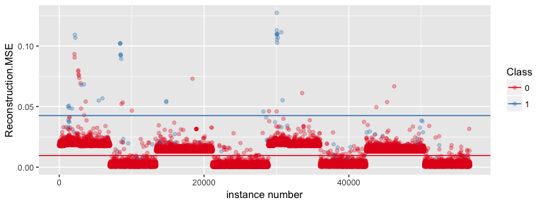
Compared to the results from yesterday’s post, this model seems to have learned a pattern that found two major cases. The mean reconstruction MSE was slightly higher for class 0 and definitely higher for class 1.
anomaly <- anomaly %>%
  mutate(outlier = ifelse(Reconstruction.MSE > 0.04, "outlier", "no_outlier"))

anomaly %>%
  group_by(Class, outlier) %>%
  summarise(n = n()) %>%
  mutate(freq = n / sum(n))
## Source: local data frame [4 x 4]
## Groups: Class [2]
##
##   Class    outlier     n         freq
##   <chr>      <chr> <int>        <dbl>
## 1     0 no_outlier 56608 0.9995762113
## 2     0    outlier    24 0.0004237887
## 3     1 no_outlier    60 0.6521739130
## 4     1    outlier    32 0.3478260870
Anomaly detection with a higher threshold based on the plot above did not improve the results compared to yesterday’s post.
With a lower threshold of 0.2 (not shown here), the test set performed much better for detecting fraud cases as outliers (65 vs 27, compared to 32 vs 60 in yesterday’s post). However, this model also categorized many more non-fraud cases as outliers (2803 vs 53829, compared to only 30 vs 56602).
Now, I am again using the autoencoder model as pre-training input for supervised learning.
model_nn_2 <- h2o.deeplearning(y = response,
                               x = features,
                               training_frame = train_supervised,
                               pretrained_autoencoder  = "model_nn",
                               reproducible = TRUE, #slow - turn off for real problems
                               balance_classes = TRUE,
                               ignore_const_cols = FALSE,
                               seed = 42,
                               hidden = c(10, 2, 10),
                               epochs = 100,
                               activation = "Tanh")
pred <- as.data.frame(h2o.predict(object = model_nn_2, newdata = test)) %>%
  mutate(actual = as.vector(test[, 31]))
pred %>%
  group_by(actual, predict) %>%
  summarise(n = n()) %>%
  mutate(freq = n / sum(n))
## Source: local data frame [4 x 4]
## Groups: actual [2]
##
##   actual predict     n       freq
##    <chr>  <fctr> <int>      <dbl>
## 1      0       0 56347 0.99496751
## 2      0       1   285 0.00503249
## 3      1       0     9 0.09782609
## 4      1       1    83 0.90217391
This model is now much better at identifying fraud cases than in yesterday’s post (90%, compared to 83% - even though we can’t directly compare the two models as they were trained on different training sets) but it is also slightly less accurate at predicting non-fraud cases (99.5%, compared to 99.8%).
If you are interested in more machine learning posts, check out the category listing for machine_learning on my blog.
sessionInfo()
## R version 3.4.0 (2017-04-21)
## Platform: x86_64-apple-darwin15.6.0 (64-bit)
## Running under: macOS Sierra 10.12.3
##
## Matrix products: default
## BLAS: /Library/Frameworks/R.framework/Versions/3.4/Resources/lib/libRblas.0.dylib
## LAPACK: /Library/Frameworks/R.framework/Versions/3.4/Resources/lib/libRlapack.dylib
##
## locale:
## [1] en_US.UTF-8/en_US.UTF-8/en_US.UTF-8/C/en_US.UTF-8/en_US.UTF-8
##
## attached base packages:
## [1] stats     graphics  grDevices utils     datasets  methods   base
##
## other attached packages:
## [1] h2o_3.10.4.4    dplyr_0.5.0     purrr_0.2.2     readr_1.1.0
## [5] tidyr_0.6.1     tibble_1.3.0    ggplot2_2.2.1   tidyverse_1.1.1
##
## loaded via a namespace (and not attached):
##  [1] Rcpp_0.12.10       RColorBrewer_1.1-2 cellranger_1.1.0
##  [4] compiler_3.4.0     plyr_1.8.4         bitops_1.0-6
##  [7] forcats_0.2.0      tools_3.4.0        digest_0.6.12
## [10] lubridate_1.6.0    jsonlite_1.4       evaluate_0.10
## [13] nlme_3.1-131       gtable_0.2.0       lattice_0.20-35
## [16] psych_1.7.3.21     DBI_0.6-1          yaml_2.1.14
## [19] parallel_3.4.0     haven_1.0.0        xml2_1.1.1
## [22] stringr_1.2.0      httr_1.2.1         knitr_1.15.1
## [25] hms_0.3            rprojroot_1.2      grid_3.4.0
## [28] R6_2.2.0           readxl_1.0.0       foreign_0.8-68
## [31] rmarkdown_1.5      modelr_0.1.0       reshape2_1.4.2
## [34] magrittr_1.5       backports_1.0.5    scales_0.4.1
## [37] htmltools_0.3.6    rvest_0.3.2        assertthat_0.2.0
## [40] mnormt_1.5-5       colorspace_1.3-2   labeling_0.3
## [43] stringi_1.1.5      RCurl_1.95-4.8     lazyeval_0.2.0
## [46] munsell_0.4.3      broom_0.4.2


