I’m an avid R user and rarely use anything else for data analysis and visualisations. But while R is my go-to, in some cases, Python might actually be a better alternative.
That’s why I wanted to see how R and Python fare in a one-on-one comparison of an analysis that’s representative of what I would typically work with.
Conclusions
All in all, the Python code could easily be translated into R and was comparable in length and simplicity between the two languages. While Python’s syntax is inherently cleaner/ tidier, we can use packages that implement piping in R and achieve similar results (even though Python’s dot-separated syntax is still much easier to type than using the piping operator of magrittr). For plotting and visualisation I still think that R’s ggplot2 is top of the line in both syntax, customizability and outcome (admittedly, I don’t know matplotlib as well as ggplot)! In terms of functionality, I couldn’t find major differences between the two languages and I would say they both have their merits. For me, R comes more natural as that is what I’m more fluent in, but I can see why Python holds an appeal too and I think I’ll make more of an effort to use both languages in my future projects.
R and Python
R and Python are both open-source languages used in a wide range of data analysis fields. Their main difference is that R has traditionally been geared towards statistical analysis, while Python is more generalist. Both comprise a large collection of packages for specific tasks and have a growing community that offers support and tutorials online.
For a nice overview of the languages respective strengths and weaknesses, check out Datacamp’s nice infographic.
Comparative analysis of genome data
To directly compare R and Python, I am following Zhuyi Xue’s “A Comprehensive Introduction To Your Genome With the SciPy Stack” (with some minor tweaks here and there). He gives a nice introduction to the data, so I will not repeat it here but focus on the comparison between the code lines.
For R, I am working with RStudio, for Python with Anaconda and Spyder.
Python:
For this analysis, we need the SciPy stack with pandas for data wrangling and matplotlib for visualisation. Anaconda already comes with all these packages that we need. Zhuyi Xue first imports pandas as “pd”, so that we can call pandas function by prefixing them with “pd.”.
import pandas as pd
R:
While the code could be replicated with base R, I prefer dplyr for data wrangling and ggplot2 for visualisation.
library(dplyr)
library(ggplot2)
Reading in data
Reading in data is straight forward in both R and Python. The code we need to read in the file is comparable between R and Python. Zhuyi Xue specified “compression = ‘gzip’”, but this would not have been necessary as the default is to infer it from the file suffix.
One big difference in the general syntax we can see here too: Boolean true/false values are written in all caps in R (TRUE/FALSE), while Python uses first letter capitalisation (True/False). The same prinicple applies to “none”.
Python:
df = pd.read_csv('Homo_sapiens.GRCh38.85.gff3.gz',
                         compression = 'gzip',
                         sep = '\t',
                         comment = '#',
                         low_memory = False,
                         header = None,
                         names = ['seqid', 'source', 'type', 'start', 'end', 'score', 'strand', 'phase', 'attributes'])
df.head()
R:
df <- read.csv("~/Documents/Github/Homo_sapiens.GRCh38.85.gff3.gz",
               header = FALSE,
               sep = "\t",
               col.names = c('seqid', 'source', 'type', 'start', 'end', 'score', 'strand', 'phase', 'attributes'),
               comment.char = "#")
head(df)
##   seqid source              type start       end   score strand phase
## 1     1 GRCh38        chromosome     1 248956422       .      .     .
## 2     1      . biological_region 10469     11240 1.3e+03      .     .
## 3     1      . biological_region 10650     10657   0.999      +     .
## 4     1      . biological_region 10655     10657   0.999      -     .
## 5     1      . biological_region 10678     10687   0.999      +     .
## 6     1      . biological_region 10681     10688   0.999      -     .
##                                           attributes
## 1 ID=chromosome:1;Alias=CM000663.2,chr1,NC_000001.11
## 2           external_name=oe %3D 0.79;logic_name=cpg
## 3                                 logic_name=eponine
## 4                                 logic_name=eponine
## 5                                 logic_name=eponine
## 6                                 logic_name=eponine
Examining data
- listing unique strings
The first thing we want to know from the data is how many unique entries there are in the “seqid” column.
Here, we can already see the main difference in syntax between R and Python:
Python concatenates the object name (“df) with the column name and the functions that we want to run on this column in a sequential manner, separated by a dot. Base R uses nested functions, where each function is called with “function_name()” and we specify columns with “object_name$column_name”.
However, both R and Python can also call columns in a dataframe with “[ ]” with the difference that Python per default subsets data columns df[“seqid”], while R always needs index specifications for rows and columns, separated by “,”: e.g. df[, “seqid”] would subset every row and only the column named “seqid”.
The sequential calling of functions is indeed very handy, it makes the code easier to read and understand than lots of interwoven functions and brackets. But while this isn’t the concept of base R, dplyr uses the magrittr principle of chaining functions with the pipe symbol “%>%”. Even though this symbol isn’t as easily typed, it’s functionality is often superior to base R, especially if you need to run many functions on a dataframe. However, with just or two functions, I usually keep to base R as it is shorter.
Python:
df.seqid.unique() # alternatively: df['seqid'].unique()
R:
unique(df$seqid)
##   [1] 1          10         11         12         13         14
##   [7] 15         16         17         18         19         2
##  [13] 20         21         22         3          4          5
##  [19] 6          7          8          9          GL000008.2 GL000009.2
##  [25] GL000194.1 GL000195.1 GL000205.2 GL000208.1 GL000213.1 GL000214.1
##  [31] GL000216.2 GL000218.1 GL000219.1 GL000220.1 GL000221.1 GL000224.1
##  [37] GL000225.1 GL000226.1 KI270302.1 KI270303.1 KI270304.1 KI270305.1
##  [43] KI270310.1 KI270311.1 KI270312.1 KI270315.1 KI270316.1 KI270317.1
##  [49] KI270320.1 KI270322.1 KI270329.1 KI270330.1 KI270333.1 KI270334.1
##  [55] KI270335.1 KI270336.1 KI270337.1 KI270338.1 KI270340.1 KI270362.1
##  [61] KI270363.1 KI270364.1 KI270366.1 KI270371.1 KI270372.1 KI270373.1
##  [67] KI270374.1 KI270375.1 KI270376.1 KI270378.1 KI270379.1 KI270381.1
##  [73] KI270382.1 KI270383.1 KI270384.1 KI270385.1 KI270386.1 KI270387.1
##  [79] KI270388.1 KI270389.1 KI270390.1 KI270391.1 KI270392.1 KI270393.1
##  [85] KI270394.1 KI270395.1 KI270396.1 KI270411.1 KI270412.1 KI270414.1
##  [91] KI270417.1 KI270418.1 KI270419.1 KI270420.1 KI270422.1 KI270423.1
##  [97] KI270424.1 KI270425.1 KI270429.1 KI270435.1 KI270438.1 KI270442.1
## [103] KI270448.1 KI270465.1 KI270466.1 KI270467.1 KI270468.1 KI270507.1
## [109] KI270508.1 KI270509.1 KI270510.1 KI270511.1 KI270512.1 KI270515.1
## [115] KI270516.1 KI270517.1 KI270518.1 KI270519.1 KI270521.1 KI270522.1
## [121] KI270528.1 KI270529.1 KI270530.1 KI270538.1 KI270539.1 KI270544.1
## [127] KI270548.1 KI270579.1 KI270580.1 KI270581.1 KI270582.1 KI270583.1
## [133] KI270584.1 KI270587.1 KI270588.1 KI270589.1 KI270590.1 KI270591.1
## [139] KI270593.1 KI270706.1 KI270707.1 KI270708.1 KI270709.1 KI270710.1
## [145] KI270711.1 KI270712.1 KI270713.1 KI270714.1 KI270715.1 KI270716.1
## [151] KI270717.1 KI270718.1 KI270719.1 KI270720.1 KI270721.1 KI270722.1
## [157] KI270723.1 KI270724.1 KI270725.1 KI270726.1 KI270727.1 KI270728.1
## [163] KI270729.1 KI270730.1 KI270731.1 KI270732.1 KI270733.1 KI270734.1
## [169] KI270735.1 KI270736.1 KI270737.1 KI270738.1 KI270739.1 KI270740.1
## [175] KI270741.1 KI270742.1 KI270743.1 KI270744.1 KI270745.1 KI270746.1
## [181] KI270747.1 KI270748.1 KI270749.1 KI270750.1 KI270751.1 KI270752.1
## [187] KI270753.1 KI270754.1 KI270755.1 KI270756.1 KI270757.1 MT
## [193] X          Y
## 194 Levels: 1 10 11 12 13 14 15 16 17 18 19 2 20 21 22 3 4 5 6 7 8 ... Y
# with dplyr:
# df %>% select(seqid) %>% unique
- how many unique seqids are there?
To get the number of unique entries in the “seqid” column, we simply need to append “.shape” to the above Python code. In R, we can either wrap the above R code with the “length()” function or use dplyr and piping instead. If we use the latter, we need to use the “nrow()” function because base R returns a vector, while dplyr returns a dataframe. Here, we can see that with two functions, using dplyr is still a bit more code but it already looks much tidier.
Python:
df.seqid.unique().shape
R:
length(unique(df$seqid))
## [1] 194
# with dplyr:
# df %>% select(seqid) %>% unique %>% nrow
- counting occurrences
To count the frequencies of each unique entry in the “source” column, we use the “value_counts()” function in Python and the “table()” function in R. These two functions differ in how they sort the output table: value_counts() sorts by decreasing frequency, while R alphabetically sorts the variables. To order the data as in Python, we need to add the “sort()” function to our R code.
Python:
df.source.value_counts()
R:
# table(df$source) is per default ordered alphabetically, if we want it ordered by decreasing counts, like with Python:
sort(table(df$source), decreasing = TRUE)
##
##         havana ensembl_havana        ensembl              .        mirbase
##        1441093         745065         228212         182510           4701
##         GRCh38          insdc
##            194             74
# dplyr:
# df %>% select(source) %>% table %>% sort(decreasing = TRUE)
How Much of the Genome Is Incomplete?
- subsetting a dataframe
We are now subsetting our original dataframe and assign it a new object name with “ = “ or “ <- “.
To subset the dataframe to keep only rows which say “GRCh38” in the “source” column, ther are several ways to do this in R: the way that would be directly comparable to how it was done in Python would be to also use the square bracket indexing. However, there are two solutions which are more elegant: 1) base R’s “subset()” or dplyr’s “filter()” function. But with this short example, there is no big difference between the three.
Python’s “shape” gives us the same information as R’s “dim()” function: how many rows and columns our dataframe has.
To preview a random subset of 10 rows from our dataframe, we use Python’s “sample()” and dplyr’s “sample_n()” function.
Python:
gdf = df[df.source == 'GRCh38']

gdf.shape
gdf.sample(10)
R:
gdf <- df[df$source == "GRCh38", ]

# alternatively:
# gdf <- subset(df, source == "GRCh38")

# dplyr:
# gdf <- df %>% filter(source == "GRCh38")

# get number of rows and columns
dim(gdf)
## [1] 194 9
# randomly sample 10 rows for observation
sample_n(gdf, 10)
##              seqid source        type start       end score strand phase
## 2511484 KI270375.1 GRCh38 supercontig     1      2378     .      .     .
## 2511545 KI270466.1 GRCh38 supercontig     1      1233     .      .     .
## 2511473 KI270337.1 GRCh38 supercontig     1      1121     .      .     .
## 2511504 KI270411.1 GRCh38 supercontig     1      2646     .      .     .
## 2511487 KI270379.1 GRCh38 supercontig     1      1045     .      .     .
## 483371          12 GRCh38  chromosome     1 133275309     .      .     .
## 2511494 KI270387.1 GRCh38 supercontig     1      1537     .      .     .
## 674768          14 GRCh38  chromosome     1 107043718     .      .     .
## 2511493 KI270386.1 GRCh38 supercontig     1      1788     .      .     .
## 2511505 KI270412.1 GRCh38 supercontig     1      1179     .      .     .
##                                                           attributes
## 2511484 ID=supercontig:KI270375.1;Alias=chrUn_KI270375v1,NT_187493.1
## 2511545 ID=supercontig:KI270466.1;Alias=chrUn_KI270466v1,NT_187421.1
## 2511473 ID=supercontig:KI270337.1;Alias=chrUn_KI270337v1,NT_187466.1
## 2511504 ID=supercontig:KI270411.1;Alias=chrUn_KI270411v1,NT_187409.1
## 2511487 ID=supercontig:KI270379.1;Alias=chrUn_KI270379v1,NT_187472.1
## 483371          ID=chromosome:12;Alias=CM000674.2,chr12,NC_000012.12
## 2511494 ID=supercontig:KI270387.1;Alias=chrUn_KI270387v1,NT_187475.1
## 674768           ID=chromosome:14;Alias=CM000676.2,chr14,NC_000014.9
## 2511493 ID=supercontig:KI270386.1;Alias=chrUn_KI270386v1,NT_187480.1
## 2511505 ID=supercontig:KI270412.1;Alias=chrUn_KI270412v1,NT_187408.1
- creating new columns and performing calculations
Now we want to create a new column called “length”. It should contain the gene lengths, i.e. the distance in base pairs between the start and end point on the chromosomes (“start” and “end” columns). In R we don’t need to copy the dataframe first but the rest of the code is very similar: we define a new column name for the dataframe and assign its value by subtracting the values of the “start” from the values of the “end” column (+1). Here, we can see again that in Python we use a dot to define columns, while R uses the Dollar sign.
The sum of all lengths is calculated with the “sum()” function in both languages.
Python:
gdf = gdf.copy()
gdf['length'] = gdf.end - gdf.start + 1

gdf.length.sum()
R:
gdf$length <- gdf$end - gdf$start + 1

sum(gdf$length)
## [1] 3096629726
Next, we want to calculating the proportion of the genome that is not on main chromosome assemblies. For that, we first define a character string with the main chromosomes: 1 to 23, X, Y and MT (mitochondrial chromosome). Defining this string is a bit easier in R.
We will use this string to calculate the sum of lengths of the subsetted dataframe and divide it by the sum of lengths of the whole dataframe. For subsetting, we use the “isin()” function of Python, which corresponds to R’s “%in%”.
Python:
chrs = [str(_) for _ in range(1, 23)] + ['X', 'Y', 'MT']
gdf[-gdf.seqid.isin(chrs)].length.sum() / gdf.length.sum()

# or
gdf[(gdf['type'] == 'supercontig')].length.sum() / gdf.length.sum()
R:
chrs <- c(1:23, "X", "Y", "MT")
sum(subset(gdf, !seqid %in% chrs)$length) / sum(gdf$length)
## [1] 0.003702192
How Many Genes Are There?
Here, we are again using the same functions as above for subsetting the dataframe, asking for its dimensions, printing 10 random lines and asking for the frequencies of each unique item in the “type” column. For the latter I am using base R over dplyr, because it’s faster to type.
Python:
edf = df[df.source.isin(['ensembl', 'havana', 'ensembl_havana'])]
edf.shape

edf.sample(10)
edf.type.value_counts()
R:
edf <- subset(df, source %in% c("ensembl", "havana", "ensembl_havana"))
dim(edf)
## [1] 2414370 9
sample_n(edf, 10)
##         seqid         source            type     start       end score
## 2548897     X        ensembl three_prime_UTR  67723842  67730618     .
## 790670     15 ensembl_havana             CDS  42352030  42352139     .
## 1298369    19         havana             CDS  38942683  38942751     .
## 189728      1 ensembl_havana             CDS 186304108 186304257     .
## 1080599    17         havana            exon  44401337  44401453     .
## 1562968    20 ensembl_havana            exon   2964272   2964350     .
## 1965100     5        ensembl      transcript    144087    144197     .
## 2581554     X         havana            exon 147927670 147928807     .
## 785399     15         havana            exon  40611478  40611511     .
## 1417830     2 ensembl_havana             CDS  71520178  71520208     .
##         strand phase
## 2548897      +     .
## 790670       +     2
## 1298369      -     0
## 189728       +     2
## 1080599      -     .
## 1562968      +     .
## 1965100      -     .
## 2581554      +     .
## 785399       +     .
## 1417830      +     0
##                                                                                                                                                                         attributes
## 2548897                                                                                                                                          Parent=transcript:ENST00000612452
## 790670                                                                                         ID=CDS:ENSP00000326227;Parent=transcript:ENST00000318010;protein_id=ENSP00000326227
## 1298369                                                                                        ID=CDS:ENSP00000472465;Parent=transcript:ENST00000599996;protein_id=ENSP00000472465
## 189728                                                                                         ID=CDS:ENSP00000356453;Parent=transcript:ENST00000367483;protein_id=ENSP00000356453
## 1080599                         Parent=transcript:ENST00000585614;Name=ENSE00002917300;constitutive=0;ensembl_end_phase=2;ensembl_phase=2;exon_id=ENSE00002917300;rank=7;version=1
## 1562968                        Parent=transcript:ENST00000216877;Name=ENSE00003603687;constitutive=1;ensembl_end_phase=1;ensembl_phase=-1;exon_id=ENSE00003603687;rank=4;version=1
## 1965100 ID=transcript:ENST00000362670;Parent=gene:ENSG00000199540;Name=Y_RNA.43-201;biotype=misc_RNA;tag=basic;transcript_id=ENST00000362670;transcript_support_level=NA;version=1
## 2581554                       Parent=transcript:ENST00000620828;Name=ENSE00003724969;constitutive=0;ensembl_end_phase=-1;ensembl_phase=-1;exon_id=ENSE00003724969;rank=1;version=1
## 785399                          Parent=transcript:ENST00000399668;Name=ENSE00003659959;constitutive=0;ensembl_end_phase=2;ensembl_phase=1;exon_id=ENSE00003659959;rank=7;version=1
## 1417830                                                                                        ID=CDS:ENSP00000398305;Parent=transcript:ENST00000429174;protein_id=ENSP00000398305
sort(table(edf$type), decreasing = TRUE)
##
##                          exon                           CDS
##                       1180596                        704604
##                five_prime_UTR               three_prime_UTR
##                        142387                        133938
##                    transcript                          gene
##                         96375                         42470
##          processed_transcript aberrant_processed_transcript
##                         28228                         26944
##        NMD_transcript_variant                       lincRNA
##                         13761                         13247
##          processed_pseudogene                  lincRNA_gene
##                         10722                          7533
##                    pseudogene                           RNA
##                          3049                          2221
##                         snRNA                    snRNA_gene
##                          1909                          1909
##                        snoRNA                   snoRNA_gene
##                           956                           944
##        pseudogenic_transcript                          rRNA
##                           737                           549
##                     rRNA_gene                         miRNA
##                           549                           302
##                V_gene_segment                J_gene_segment
##                           216                           158
##               VD_gene_segment                C_gene_segment
##                            37                            29
##             biological_region                    chromosome
##                             0                             0
##                    miRNA_gene                       mt_gene
##                             0                             0
##                   supercontig
##                             0
Now we want to subset the dataframe to rows with the attribute “gene” in the “type” column, look at 10 random lines from the “attributes” column and get the dataframe dimensions.
Python:
ndf = edf[edf.type == 'gene']
ndf = ndf.copy()
ndf.sample(10).attributes.values
ndf.shape
R:
ndf <- subset(edf, type == "gene")
sample_n(ndf, 10)$attributes
##  [1] ID=gene:ENSG00000170949;Name=ZNF160;biotype=protein_coding;description=zinc finger protein 160 [Source:HGNC Symbol%3BAcc:HGNC:12948];gene_id=ENSG00000170949;havana_gene=OTTHUMG00000182854;havana_version=3;logic_name=ensembl_havana_gene;version=17
##  [2] ID=gene:ENSG00000215088;Name=RPS5P3;biotype=processed_pseudogene;description=ribosomal protein S5 pseudogene 3 [Source:HGNC Symbol%3BAcc:HGNC:10427];gene_id=ENSG00000215088;havana_gene=OTTHUMG00000065532;havana_version=1;logic_name=havana;version=3
##  [3] ID=gene:ENSG00000249077;Name=RP11-478C1.8;biotype=processed_pseudogene;gene_id=ENSG00000249077;havana_gene=OTTHUMG00000160290;havana_version=1;logic_name=havana;version=1
##  [4] ID=gene:ENSG00000110619;Name=CARS;biotype=protein_coding;description=cysteinyl-tRNA synthetase [Source:HGNC Symbol%3BAcc:HGNC:1493];gene_id=ENSG00000110619;havana_gene=OTTHUMG00000010927;havana_version=9;logic_name=ensembl_havana_gene;version=16
##  [5] ID=gene:ENSG00000168010;Name=ATG16L2;biotype=protein_coding;description=autophagy related 16 like 2 [Source:HGNC Symbol%3BAcc:HGNC:25464];gene_id=ENSG00000168010;havana_gene=OTTHUMG00000167961;havana_version=2;logic_name=ensembl_havana_gene;version=10
##  [6] ID=gene:ENSG00000055957;Name=ITIH1;biotype=protein_coding;description=inter-alpha-trypsin inhibitor heavy chain 1 [Source:HGNC Symbol%3BAcc:HGNC:6166];gene_id=ENSG00000055957;havana_gene=OTTHUMG00000150312;havana_version=9;logic_name=ensembl_havana_gene;version=10
##  [7] ID=gene:ENSG00000258781;Name=RP11-496I2.4;biotype=unprocessed_pseudogene;gene_id=ENSG00000258781;havana_gene=OTTHUMG00000170502;havana_version=2;logic_name=havana;version=2
##  [8] ID=gene:ENSG00000157965;Name=SSX8;biotype=unprocessed_pseudogene;description=SSX family member 8 [Source:HGNC Symbol%3BAcc:HGNC:19654];gene_id=ENSG00000157965;havana_gene=OTTHUMG00000021573;havana_version=4;logic_name=havana;version=11
##  [9] ID=gene:ENSG00000273489;Name=RP11-180C16.1;biotype=antisense;gene_id=ENSG00000273489;havana_gene=OTTHUMG00000186336;havana_version=1;logic_name=havana;version=1
## [10] ID=gene:ENSG00000279532;Name=CTB-96E2.6;biotype=TEC;gene_id=ENSG00000279532;havana_gene=OTTHUMG00000179414;havana_version=1;logic_name=havana;version=1
## 1623077 Levels: external_name=Ala;logic_name=trnascan ...
dim(ndf)
## [1] 42470 9
- extracting gene information from attributes field
I don’t know if there is an easier way in Python but in R we don’t need to create big helper functions around it. We can simply use “gsub()” with defining the regular expression for what we want to extract. This makes the R code much shorter and easier to understand! We then drop the original “attributes” column.
To have a look at the dataframe, we use “head()” this time.
Python:
import re

RE_GENE_NAME = re.compile(r'Name=(?P<gene_name>.+?);')
def extract_gene_name(attributes_str):
    res = RE_GENE_NAME.search(attributes_str)
    return res.group('gene_name')


ndf['gene_name'] = ndf.attributes.apply(extract_gene_name)

RE_GENE_ID = re.compile(r'gene_id=(?P<gene_id>ENSG.+?);')
def extract_gene_id(attributes_str):
    res = RE_GENE_ID.search(attributes_str)
    return res.group('gene_id')


ndf['gene_id'] = ndf.attributes.apply(extract_gene_id)


RE_DESC = re.compile('description=(?P<desc>.+?);')
def extract_description(attributes_str):
    res = RE_DESC.search(attributes_str)
    if res is None:
        return ''
    else:
        return res.group('desc')


ndf['desc'] = ndf.attributes.apply(extract_description)

ndf.drop('attributes', axis=1, inplace=True)
ndf.head()
R:
ndf$gene_name <- gsub("(.*Name=)(.*?)(;biotype.*)", "\\2", ndf$attributes)
ndf$gene_id <- gsub("(ID=gene:)(.*?)(;Name.*)", "\\2", ndf$attributes)
ndf$desc <- gsub("(.*description=)(.*?)(;.*)", "\\2", ndf$attributes)

# some genes don't have a description
ndf$desc <- ifelse(grepl("^ID=.*", ndf$desc), "", ndf$desc)

ndf <- subset(ndf, select = -attributes)
head(ndf)
##     seqid         source type  start    end score strand phase gene_name
## 17      1         havana gene  11869  14409     .      +     .   DDX11L1
## 29      1         havana gene  14404  29570     .      -     .    WASH7P
## 72      1         havana gene  52473  53312     .      +     .    OR4G4P
## 75      1         havana gene  62948  63887     .      +     .   OR4G11P
## 78      1 ensembl_havana gene  69091  70008     .      +     .     OR4F5
## 109     1         havana gene 131025 134836     .      +     .    CICP27
##             gene_id
## 17  ENSG00000223972
## 29  ENSG00000227232
## 72  ENSG00000268020
## 75  ENSG00000240361
## 78  ENSG00000186092
## 109 ENSG00000233750
##                                                                                                   desc
## 17                                 DEAD/H-box helicase 11 like 1 [Source:HGNC Symbol%3BAcc:HGNC:37102]
## 29                       WAS protein family homolog 7 pseudogene [Source:HGNC Symbol%3BAcc:HGNC:38034]
## 72   olfactory receptor family 4 subfamily G member 4 pseudogene [Source:HGNC Symbol%3BAcc:HGNC:14822]
## 75  olfactory receptor family 4 subfamily G member 11 pseudogene [Source:HGNC Symbol%3BAcc:HGNC:31276]
## 78              olfactory receptor family 4 subfamily F member 5 [Source:HGNC Symbol%3BAcc:HGNC:14825]
## 109              capicua transcriptional repressor pseudogene 27 [Source:HGNC Symbol%3BAcc:HGNC:48835]
Next, we want to know how many unique gene names and gene IDs there are. As above we use the “unique()”, “shape()” (Python) and “length()” (R) functions.
The count table for gene names can again be obtained with R’s “table()” function, even though Zhuyi Xue uses a slightly different approach: he first groups the “gene_name” column, then counts and sorts.
Finally, we can calculate the proportion of genes that have more than appear more than once and we can have a closer look at the SCARNA20 gene.
Python:
ndf.shape
ndf.gene_id.unique().shape
ndf.gene_name.unique().shape

count_df = ndf.groupby('gene_name').count().ix[:, 0].sort_values().ix[::-1]
count_df.head(10)

count_df[count_df > 1].shape
count_df.shape
count_df[count_df > 1].shape[0] / count_df.shape[0]

ndf[ndf.gene_name == 'SCARNA20']
R:
dim(ndf)
## [1] 42470 11
length(unique(ndf$gene_id))
## [1] 42470
length(unique(ndf$gene_name))
## [1] 42387
count_df <- sort(table(ndf$gene_name), decreasing = TRUE)
head(count_df, n = 10)
##
##        SCARNA20        SCARNA16        SCARNA17        SCARNA11
##               7               6               5               4
##        SCARNA15        SCARNA21 Clostridiales-1         SCARNA4
##               4               4               3               3
##        ACTR3BP2           AGBL1
##               2               2
length(count_df[count_df > 1])
## [1] 63
length(count_df)
## [1] 42387
length(count_df[count_df > 1]) / length(count_df)
## [1] 0.001486305
ndf[ndf$gene_name == "SCARNA20", ]
##         seqid  source type     start       end score strand phase
## 179400      1 ensembl gene 171768070 171768175     .      +     .
## 201038      1 ensembl gene 204727991 204728106     .      +     .
## 349204     11 ensembl gene   8555016   8555146     .      +     .
## 718521     14 ensembl gene  63479272  63479413     .      +     .
## 837234     15 ensembl gene  75121536  75121666     .      -     .
## 1039875    17 ensembl gene  28018770  28018907     .      +     .
## 1108216    17 ensembl gene  60231516  60231646     .      -     .
##         gene_name         gene_id
## 179400   SCARNA20 ENSG00000253060
## 201038   SCARNA20 ENSG00000251861
## 349204   SCARNA20 ENSG00000252778
## 718521   SCARNA20 ENSG00000252800
## 837234   SCARNA20 ENSG00000252722
## 1039875  SCARNA20 ENSG00000251818
## 1108216  SCARNA20 ENSG00000252577
##                                                                           desc
## 179400            Small Cajal body specific RNA 20 [Source:RFAM%3BAcc:RF00601]
## 201038            Small Cajal body specific RNA 20 [Source:RFAM%3BAcc:RF00601]
## 349204            Small Cajal body specific RNA 20 [Source:RFAM%3BAcc:RF00601]
## 718521            Small Cajal body specific RNA 20 [Source:RFAM%3BAcc:RF00601]
## 837234            Small Cajal body specific RNA 20 [Source:RFAM%3BAcc:RF00601]
## 1039875           Small Cajal body specific RNA 20 [Source:RFAM%3BAcc:RF00601]
## 1108216 small Cajal body-specific RNA 20 [Source:HGNC Symbol%3BAcc:HGNC:32578]
# dplyr:
# ndf %>% filter(gene_name == "SCARNA20")
How Long Is a Typical Gene?
To calculate gene lengths we use the same code as before. R’s summary() is not exactly the same as Python’s describe() but it’s close enough.
Python:
ndf['length'] = ndf.end - ndf.start + 1
ndf.length.describe()
R:
ndf$length <- ndf$end - ndf$start + 1
summary(ndf$length)
##    Min. 1st Qu.  Median    Mean 3rd Qu.    Max.
##       8     884    5170   35830   30550 2305000
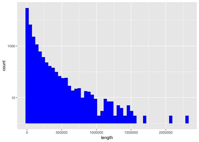
Now we produce the first plot, showing a histogram of gene length. In base R you can’t really plot a histogram with logarithmic y-axis scales (at least not without manually tweaking the hist() output but it isn’t recommended anyway because 0 will become -Inf). But we can do it easily with ggplot2 with “scale_y_log10()”. The code we need for ggplot2 is a bit longer than with matplotlib. We could of course further customize our plot but for now, let’s keep it simple.
Python:
import matplotlib as plt

ndf.length.plot(kind='hist', bins=50, logy=True)
plt.show()
R:
ndf %>% ggplot(aes(x = length)) +
  geom_histogram(bins = 50, fill = "blue") +
  scale_y_log10()
Now, we subset the dataframe to keep only rows where the “length” column contains values bigger than 2 million and order it by descending gene length. To see the shortest genes, we order the original dataframe and view the first 6 rows. Instead of “sort()”, we use dplyr’s “arrange()” function this time (I didn’t use it before because it can only be applied to dataframes).
Python:
ndf[ndf.length > 2e6].sort_values('length').ix[::-1]
ndf.sort_values('length').head()
R:
ndf %>% filter(length > 2e6) %>% arrange(desc(length))
##   seqid         source type     start       end score strand phase
## 1     7 ensembl_havana gene 146116002 148420998     .      +     .
## 2     9 ensembl_havana gene   8314246  10612723     .      -     .
## 3     X ensembl_havana gene  31097677  33339441     .      -     .
## 4    11 ensembl_havana gene  83455012  85627922     .      -     .
## 5     8 ensembl_havana gene   2935353   4994972     .      -     .
## 6    20 ensembl_havana gene  13995369  16053197     .      +     .
##   gene_name         gene_id
## 1   CNTNAP2 ENSG00000174469
## 2     PTPRD ENSG00000153707
## 3       DMD ENSG00000198947
## 4      DLG2 ENSG00000150672
## 5     CSMD1 ENSG00000183117
## 6   MACROD2 ENSG00000172264
##                                                                                   desc
## 1            contactin associated protein-like 2 [Source:HGNC Symbol%3BAcc:HGNC:13830]
## 2 protein tyrosine phosphatase%2C receptor type D [Source:HGNC Symbol%3BAcc:HGNC:9668]
## 3                                      dystrophin [Source:HGNC Symbol%3BAcc:HGNC:2928]
## 4            discs large MAGUK scaffold protein 2 [Source:HGNC Symbol%3BAcc:HGNC:2901]
## 5               CUB and Sushi multiple domains 1 [Source:HGNC Symbol%3BAcc:HGNC:14026]
## 6                      MACRO domain containing 2 [Source:HGNC Symbol%3BAcc:HGNC:16126]
##    length
## 1 2304997
## 2 2298478
## 3 2241765
## 4 2172911
## 5 2059620
## 6 2057829
head(arrange(ndf, length))
##   seqid source type     start       end score strand phase    gene_name
## 1    14 havana gene  22438547  22438554     .      +     .        TRDD1
## 2    14 havana gene  22439007  22439015     .      +     .        TRDD2
## 3     7 havana gene 142786213 142786224     .      +     .        TRBD1
## 4    14 havana gene  22449113  22449125     .      +     .        TRDD3
## 5     4 havana gene  10238213  10238235     .      -     .   AC006499.9
## 6     3 havana gene 179452395 179452419     .      -     . RP11-145M9.2
##           gene_id
## 1 ENSG00000223997
## 2 ENSG00000237235
## 3 ENSG00000282431
## 4 ENSG00000228985
## 5 ENSG00000271544
## 6 ENSG00000239255
##                                                                      desc
## 1 T cell receptor delta diversity 1 [Source:HGNC Symbol%3BAcc:HGNC:12254]
## 2 T cell receptor delta diversity 2 [Source:HGNC Symbol%3BAcc:HGNC:12255]
## 3  T cell receptor beta diversity 1 [Source:HGNC Symbol%3BAcc:HGNC:12158]
## 4 T cell receptor delta diversity 3 [Source:HGNC Symbol%3BAcc:HGNC:12256]
## 5
## 6
##   length
## 1      8
## 2      9
## 3     12
## 4     13
## 5     23
## 6     25
Gene Distribution Among Chromosomes
The number of genes per chromosome are counted with the “subset()”, “table()” and “sort()” functions as described earlier.
Python:
ndf = ndf[ndf.seqid.isin(chrs)]
chr_gene_counts = ndf.groupby('seqid').count().ix[:, 0].sort_values().ix[::-1]
chr_gene_counts
R:
ndf$seqid <- as.character(ndf$seqid) # as factors it will subset the dataframe but keep the factor levels
ndf <- subset(ndf, seqid %in% chrs)
chr_gene_counts <- sort(table(ndf$seqid), decreasing = TRUE)
chr_gene_counts
##
##    1    2   11   19   17    3    6   12    7    5   16    X    4    9    8
## 3902 2806 2561 2412 2280 2204 2154 2140 2106 2002 1881 1852 1751 1659 1628
##   10   15   14   22   20   13   18   21    Y
## 1600 1476 1449  996  965  872  766  541  436
To see all genes that are on mitochondrial chromosome, we subset the first dataframe by two conditions. In both, R and Python this is done with the ampersand symbol but in R we don’t need brackets around the individual conditions.
Python:
df[(df.type == 'gene') & (df.seqid == 'MT')]
R:
subset(df, type == "gene" & seqid == "MT")
##         seqid source type start   end score strand phase
## 2514004    MT  insdc gene   648  1601     .      +     .
## 2514010    MT  insdc gene  1671  3229     .      +     .
## 2514017    MT  insdc gene  3307  4262     .      +     .
## 2514030    MT  insdc gene  4470  5511     .      +     .
## 2514049    MT  insdc gene  5904  7445     .      +     .
## 2514059    MT  insdc gene  7586  8269     .      +     .
## 2514066    MT  insdc gene  8366  8572     .      +     .
## 2514070    MT  insdc gene  8527  9207     .      +     .
## 2514074    MT  insdc gene  9207  9990     .      +     .
## 2514081    MT  insdc gene 10059 10404     .      +     .
## 2514088    MT  insdc gene 10470 10766     .      +     .
## 2514092    MT  insdc gene 10760 12137     .      +     .
## 2514105    MT  insdc gene 12337 14148     .      +     .
## 2514109    MT  insdc gene 14149 14673     .      -     .
## 2514116    MT  insdc gene 14747 15887     .      +     .
##                                                                                                                                                                                                                                                 attributes
## 2514004                                               ID=gene:ENSG00000211459;Name=MT-RNR1;biotype=Mt_rRNA;description=mitochondrially encoded 12S RNA [Source:HGNC Symbol%3BAcc:HGNC:7470];gene_id=ENSG00000211459;logic_name=mt_genbank_import;version=2
## 2514010                                               ID=gene:ENSG00000210082;Name=MT-RNR2;biotype=Mt_rRNA;description=mitochondrially encoded 16S RNA [Source:HGNC Symbol%3BAcc:HGNC:7471];gene_id=ENSG00000210082;logic_name=mt_genbank_import;version=2
## 2514017   ID=gene:ENSG00000198888;Name=MT-ND1;biotype=protein_coding;description=mitochondrially encoded NADH:ubiquinone oxidoreductase core subunit 1 [Source:HGNC Symbol%3BAcc:HGNC:7455];gene_id=ENSG00000198888;logic_name=mt_genbank_import;version=2
## 2514030   ID=gene:ENSG00000198763;Name=MT-ND2;biotype=protein_coding;description=mitochondrially encoded NADH:ubiquinone oxidoreductase core subunit 2 [Source:HGNC Symbol%3BAcc:HGNC:7456];gene_id=ENSG00000198763;logic_name=mt_genbank_import;version=3
## 2514049                          ID=gene:ENSG00000198804;Name=MT-CO1;biotype=protein_coding;description=mitochondrially encoded cytochrome c oxidase I [Source:HGNC Symbol%3BAcc:HGNC:7419];gene_id=ENSG00000198804;logic_name=mt_genbank_import;version=2
## 2514059                         ID=gene:ENSG00000198712;Name=MT-CO2;biotype=protein_coding;description=mitochondrially encoded cytochrome c oxidase II [Source:HGNC Symbol%3BAcc:HGNC:7421];gene_id=ENSG00000198712;logic_name=mt_genbank_import;version=1
## 2514066                                 ID=gene:ENSG00000228253;Name=MT-ATP8;biotype=protein_coding;description=mitochondrially encoded ATP synthase 8 [Source:HGNC Symbol%3BAcc:HGNC:7415];gene_id=ENSG00000228253;logic_name=mt_genbank_import;version=1
## 2514070                                 ID=gene:ENSG00000198899;Name=MT-ATP6;biotype=protein_coding;description=mitochondrially encoded ATP synthase 6 [Source:HGNC Symbol%3BAcc:HGNC:7414];gene_id=ENSG00000198899;logic_name=mt_genbank_import;version=2
## 2514074                        ID=gene:ENSG00000198938;Name=MT-CO3;biotype=protein_coding;description=mitochondrially encoded cytochrome c oxidase III [Source:HGNC Symbol%3BAcc:HGNC:7422];gene_id=ENSG00000198938;logic_name=mt_genbank_import;version=2
## 2514081   ID=gene:ENSG00000198840;Name=MT-ND3;biotype=protein_coding;description=mitochondrially encoded NADH:ubiquinone oxidoreductase core subunit 3 [Source:HGNC Symbol%3BAcc:HGNC:7458];gene_id=ENSG00000198840;logic_name=mt_genbank_import;version=2
## 2514088 ID=gene:ENSG00000212907;Name=MT-ND4L;biotype=protein_coding;description=mitochondrially encoded NADH:ubiquinone oxidoreductase core subunit 4L [Source:HGNC Symbol%3BAcc:HGNC:7460];gene_id=ENSG00000212907;logic_name=mt_genbank_import;version=2
## 2514092   ID=gene:ENSG00000198886;Name=MT-ND4;biotype=protein_coding;description=mitochondrially encoded NADH:ubiquinone oxidoreductase core subunit 4 [Source:HGNC Symbol%3BAcc:HGNC:7459];gene_id=ENSG00000198886;logic_name=mt_genbank_import;version=2
## 2514105   ID=gene:ENSG00000198786;Name=MT-ND5;biotype=protein_coding;description=mitochondrially encoded NADH:ubiquinone oxidoreductase core subunit 5 [Source:HGNC Symbol%3BAcc:HGNC:7461];gene_id=ENSG00000198786;logic_name=mt_genbank_import;version=2
## 2514109   ID=gene:ENSG00000198695;Name=MT-ND6;biotype=protein_coding;description=mitochondrially encoded NADH:ubiquinone oxidoreductase core subunit 6 [Source:HGNC Symbol%3BAcc:HGNC:7462];gene_id=ENSG00000198695;logic_name=mt_genbank_import;version=2
## 2514116                                    ID=gene:ENSG00000198727;Name=MT-CYB;biotype=protein_coding;description=mitochondrially encoded cytochrome b [Source:HGNC Symbol%3BAcc:HGNC:7427];gene_id=ENSG00000198727;logic_name=mt_genbank_import;version=2
We can get the chromosome lengths from the dataframe as well. We again subset to only the main chromosomes, then drop unwanted columns and order by length.
Python:
gdf = gdf[gdf.seqid.isin(chrs)]
gdf.drop(['start', 'end', 'score', 'strand', 'phase' ,'attributes'], axis=1, inplace=True)
gdf.sort_values('length').ix[::-1]
R:
gdf$seqid <- as.character(gdf$seqid) # as factors it will subset the dataframe but keep the factor levels
gdf <- subset(gdf, as.character(seqid) %in% chrs) %>%
  select(-(start:attributes))
arrange(gdf, desc(length))
##    seqid source       type    length
## 1      1 GRCh38 chromosome 248956422
## 2      2 GRCh38 chromosome 242193529
## 3      3 GRCh38 chromosome 198295559
## 4      4 GRCh38 chromosome 190214555
## 5      5 GRCh38 chromosome 181538259
## 6      6 GRCh38 chromosome 170805979
## 7      7 GRCh38 chromosome 159345973
## 8      X GRCh38 chromosome 156040895
## 9      8 GRCh38 chromosome 145138636
## 10     9 GRCh38 chromosome 138394717
## 11    11 GRCh38 chromosome 135086622
## 12    10 GRCh38 chromosome 133797422
## 13    12 GRCh38 chromosome 133275309
## 14    13 GRCh38 chromosome 114364328
## 15    14 GRCh38 chromosome 107043718
## 16    15 GRCh38 chromosome 101991189
## 17    16 GRCh38 chromosome  90338345
## 18    17 GRCh38 chromosome  83257441
## 19    18 GRCh38 chromosome  80373285
## 20    20 GRCh38 chromosome  64444167
## 21    19 GRCh38 chromosome  58617616
## 22     Y GRCh38 chromosome  54106423
## 23    22 GRCh38 chromosome  50818468
## 24    21 GRCh38 chromosome  46709983
## 25    MT GRCh38 chromosome     16569
Now, we merge the dataframe with the number of genes per chromosome with the dataframe of chromosome lengths. Because R’s “table()” function produces a vector, we need to convert it to a dataframe first and define the column names. Then, we use the “merge()” function and point to the name of the column we want to merge by.
Python:
cdf = chr_gene_counts.to_frame(name='gene_count').reset_index()
cdf.head(2)

merged = gdf.merge(cdf, on='seqid')
R:
cdf <- as.data.frame(chr_gene_counts)
colnames(cdf) <- c("seqid", "gene_count")
head(cdf, n = 2)
##   seqid gene_count
## 1     1       3902
## 2     2       2806
merged <- merge(gdf, cdf, by = "seqid")
merged
##    seqid source       type    length gene_count
## 1      1 GRCh38 chromosome 248956422       3902
## 2     10 GRCh38 chromosome 133797422       1600
## 3     11 GRCh38 chromosome 135086622       2561
## 4     12 GRCh38 chromosome 133275309       2140
## 5     13 GRCh38 chromosome 114364328        872
## 6     14 GRCh38 chromosome 107043718       1449
## 7     15 GRCh38 chromosome 101991189       1476
## 8     16 GRCh38 chromosome  90338345       1881
## 9     17 GRCh38 chromosome  83257441       2280
## 10    18 GRCh38 chromosome  80373285        766
## 11    19 GRCh38 chromosome  58617616       2412
## 12     2 GRCh38 chromosome 242193529       2806
## 13    20 GRCh38 chromosome  64444167        965
## 14    21 GRCh38 chromosome  46709983        541
## 15    22 GRCh38 chromosome  50818468        996
## 16     3 GRCh38 chromosome 198295559       2204
## 17     4 GRCh38 chromosome 190214555       1751
## 18     5 GRCh38 chromosome 181538259       2002
## 19     6 GRCh38 chromosome 170805979       2154
## 20     7 GRCh38 chromosome 159345973       2106
## 21     8 GRCh38 chromosome 145138636       1628
## 22     9 GRCh38 chromosome 138394717       1659
## 23     X GRCh38 chromosome 156040895       1852
## 24     Y GRCh38 chromosome  54106423        436
To calculate the correlation between length and gene count, we subset the merged dataframe to those two columns and use the “corr()” (Python) or “cor()” (R) function.
Python:
merged[['length', 'gene_count']].corr()
R:
cor(merged[, c("length", "gene_count")])
##               length gene_count
## length     1.0000000  0.7282208
## gene_count 0.7282208  1.0000000
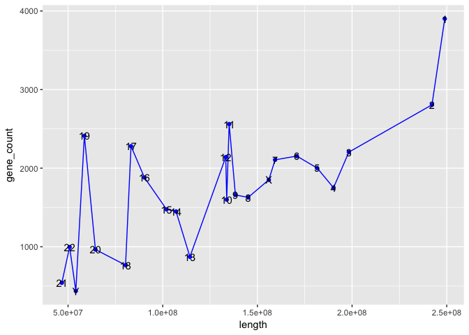
And now we produce the final plot: a line plot of chromosome length by number of genes per chromosome. For Python, we again use the matplotlib and for R the ggplot2 packages. Because Zhuyi Xue creates a new dataframe and tweaks the plot somewhat, our ggplot2 code is simpler and tidier here.
Python:
ax = merged[['length', 'gene_count']].sort_values('length').plot(x='length', y='gene_count', style='o-')
# add some margin to both ends of x axis
xlim = ax.get_xlim()
margin = xlim[0] * 0.1
ax.set_xlim([xlim[0] - margin, xlim[1] + margin])
# Label each point on the graph
for (s, x, y) in merged[['seqid', 'length', 'gene_count']].sort_values('length').values:
    ax.text(x, y - 100, str(s))
R:
merged[, c("seqid", "length", "gene_count")] %>%
  arrange(desc(length)) %>%
  ggplot(aes(x = length, y = gene_count, label = seqid)) +
  geom_point(color = "blue") +
  geom_line(color = "blue") +
  geom_text()
## R version 3.3.2 (2016-10-31)
## Platform: x86_64-apple-darwin13.4.0 (64-bit)
## Running under: macOS Sierra 10.12.1
##
## locale:
## [1] en_US.UTF-8/en_US.UTF-8/en_US.UTF-8/C/en_US.UTF-8/en_US.UTF-8
##
## attached base packages:
## [1] stats     graphics  grDevices utils     datasets  methods   base
##
## other attached packages:
## [1] ggplot2_2.2.1 dplyr_0.5.0
##
## loaded via a namespace (and not attached):
##  [1] Rcpp_0.12.8      codetools_0.2-15 digest_0.6.11    rprojroot_1.1
##  [5] assertthat_0.1   plyr_1.8.4       grid_3.3.2       R6_2.2.0
##  [9] gtable_0.2.0     DBI_0.5-1        backports_1.0.4  magrittr_1.5
## [13] scales_0.4.1     evaluate_0.10    stringi_1.1.2    lazyeval_0.2.0
## [17] rmarkdown_1.3    labeling_0.3     tools_3.3.2      stringr_1.1.0
## [21] munsell_0.4.3    yaml_2.1.14      colorspace_1.3-2 htmltools_0.3.5
## [25] knitr_1.15.1     tibble_1.2