Edited on 26 December 2016
Among the many R packages, there is the outbreaks package. It contains datasets on epidemics, on of which is from the 2013 outbreak of influenza A H7N9 in China, as analysed by Kucharski et al. (2014):
A. Kucharski, H. Mills, A. Pinsent, C. Fraser, M. Van Kerkhove, C. A. Donnelly, and S. Riley. 2014. Distinguishing between reservoir exposure and human-to-human transmission for emerging pathogens using case onset data. PLOS Currents Outbreaks. Mar 7, edition 1. doi: 10.1371/currents.outbreaks.e1473d9bfc99d080ca242139a06c455f.
A. Kucharski, H. Mills, A. Pinsent, C. Fraser, M. Van Kerkhove, C. A. Donnelly, and S. Riley. 2014. Data from: Distinguishing between reservoir exposure and human-to-human transmission for emerging pathogens using case onset data. Dryad Digital Repository. http://dx.doi.org/10.5061/dryad.2g43n.
I will be using their data as an example to test whether we can use Machine Learning algorithms for predicting disease outcome.
To do so, I selected and extracted features from the raw data, including age, days between onset and outcome, gender, whether the patients were hospitalised, etc. Missing values were imputed and different model algorithms were used to predict outcome (death or recovery). The prediction accuracy, sensitivity and specificity. The thus prepared dataset was devided into training and testing subsets. The test subset contained all cases with an unknown outcome. Before I applied the models to the test data, I further split the training data into validation subsets.
The tested modeling algorithms were similarly successful at predicting the outcomes of the validation data. To decide on final classifications, I compared predictions from all models and defined the outcome “Death” or “Recovery” as a function of all models, whereas classifications with a low prediction probability were flagged as “uncertain”. Accounting for this uncertainty led to a 100% correct classification of the validation test set.
The training cases with unknown outcome were then classified based on the same algorithms. From 57 unknown cases, 14 were classified as “Recovery”, 10 as “Death” and 33 as uncertain.
In a Part 2 I am looking at how extreme gradient boosting performs on this dataset.
The data
The dataset contains case ID, date of onset, date of hospitalisation, date of outcome, gender, age, province and of course the outcome: Death or Recovery. I can already see that there are a couple of missing values in the data, which I will deal with later.
# install and load package
if (!require("outbreaks")) install.packages("outbreaks")
library(outbreaks)
fluH7N9.china.2013_backup <- fluH7N9.china.2013 # back up original dataset in case something goes awry along the way

# convert ? to NAs
fluH7N9.china.2013$age[which(fluH7N9.china.2013$age == "?")] <- NA

# create a new column with case ID
fluH7N9.china.2013$case.ID <- paste("case", fluH7N9.china.2013$case.ID, sep = "_")
head(fluH7N9.china.2013)
##   case.ID date.of.onset date.of.hospitalisation date.of.outcome outcome gender age province
## 1  case_1    2013-02-19                    <NA>      2013-03-04   Death      m  87 Shanghai
## 2  case_2    2013-02-27              2013-03-03      2013-03-10   Death      m  27 Shanghai
## 3  case_3    2013-03-09              2013-03-19      2013-04-09   Death      f  35    Anhui
## 4  case_4    2013-03-19              2013-03-27            <NA>    <NA>      f  45  Jiangsu
## 5  case_5    2013-03-19              2013-03-30      2013-05-15 Recover      f  48  Jiangsu
## 6  case_6    2013-03-21              2013-03-28      2013-04-26   Death      f  32  Jiangsu
Before I start preparing the data for Machine Learning, I want to get an idea of the distribution of the data points and their different variables by plotting.
Most provinces have only a handful of cases, so I am combining them into the category “other” and keep only Jiangsu, Shanghai and Zhejian and separate provinces.
# gather for plotting with ggplot2
library(tidyr)
fluH7N9.china.2013_gather <- fluH7N9.china.2013 %>%
  gather(Group, Date, date.of.onset:date.of.outcome)

# rearrange group order
fluH7N9.china.2013_gather$Group <- factor(fluH7N9.china.2013_gather$Group, levels = c("date.of.onset", "date.of.hospitalisation", "date.of.outcome"))

# rename groups
library(plyr)
fluH7N9.china.2013_gather$Group <- mapvalues(fluH7N9.china.2013_gather$Group, from = c("date.of.onset", "date.of.hospitalisation", "date.of.outcome"),
          to = c("Date of onset", "Date of hospitalisation", "Date of outcome"))

# renaming provinces
fluH7N9.china.2013_gather$province <- mapvalues(fluH7N9.china.2013_gather$province,
                                                from = c("Anhui", "Beijing", "Fujian", "Guangdong", "Hebei", "Henan", "Hunan", "Jiangxi", "Shandong", "Taiwan"),
                                                to = rep("Other", 10))

# add a level for unknown gender
levels(fluH7N9.china.2013_gather$gender) <- c(levels(fluH7N9.china.2013_gather$gender), "unknown")
fluH7N9.china.2013_gather$gender[is.na(fluH7N9.china.2013_gather$gender)] <- "unknown"

# rearrange province order so that Other is the last
fluH7N9.china.2013_gather$province <- factor(fluH7N9.china.2013_gather$province, levels = c("Jiangsu",  "Shanghai", "Zhejiang", "Other"))

# convert age to numeric
fluH7N9.china.2013_gather$age <- as.numeric(as.character(fluH7N9.china.2013_gather$age))
# preparing my ggplot2 theme of choice

library(ggplot2)
my_theme <- function(base_size = 12, base_family = "sans"){
  theme_minimal(base_size = base_size, base_family = base_family) +
  theme(
    axis.text = element_text(size = 12),
    axis.text.x = element_text(angle = 45, vjust = 0.5, hjust = 0.5),
    axis.title = element_text(size = 14),
    panel.grid.major = element_line(color = "grey"),
    panel.grid.minor = element_blank(),
    panel.background = element_rect(fill = "aliceblue"),
    strip.background = element_rect(fill = "lightgrey", color = "grey", size = 1),
    strip.text = element_text(face = "bold", size = 12, color = "black"),
    legend.position = "bottom",
    legend.justification = "top",
    legend.box = "horizontal",
    legend.box.background = element_rect(colour = "grey50"),
    legend.background = element_blank(),
    panel.border = element_rect(color = "grey", fill = NA, size = 0.5)
  )
}
# plotting raw data

ggplot(data = fluH7N9.china.2013_gather, aes(x = Date, y = age, fill = outcome)) +
  stat_density2d(aes(alpha = ..level..), geom = "polygon") +
  geom_jitter(aes(color = outcome, shape = gender), size = 1.5) +
  geom_rug(aes(color = outcome)) +
  labs(
    fill = "Outcome",
    color = "Outcome",
    alpha = "Level",
    shape = "Gender",
    x = "Date in 2013",
    y = "Age",
    title = "2013 Influenza A H7N9 cases in China",
    subtitle = "Dataset from 'outbreaks' package (Kucharski et al. 2014)",
    caption = ""
  ) +
  facet_grid(Group ~ province) +
  my_theme() +
  scale_shape_manual(values = c(15, 16, 17)) +
  scale_color_brewer(palette="Set1", na.value = "grey50") +
  scale_fill_brewer(palette="Set1")
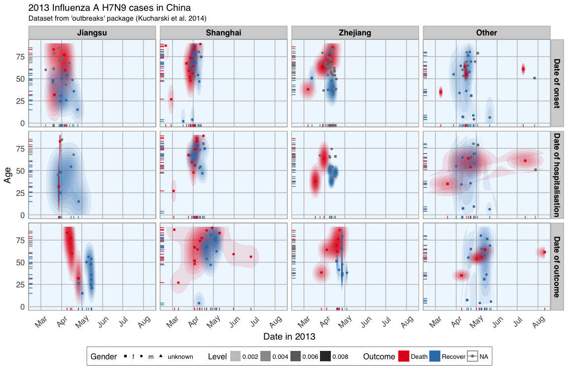
This plot shows the dates of onset, hospitalisation and outcome (if known) of each data point. Outcome is marked by color and age shown on the y-axis. Gender is marked by point shape.
The density distribution of date by age for the cases seems to indicate that older people died more frequently in the Jiangsu and Zhejiang province than in Shanghai and in other provinces.
When we look at the distribution of points along the time axis, it suggests that their might be a positive correlation between the likelihood of death and an early onset or early outcome.
I also want to know how many cases there are for each gender and province and compare the genders’ age distribution.
fluH7N9.china.2013_gather_2 <- fluH7N9.china.2013_gather[, -4] %>%
  gather(group_2, value, gender:province)

fluH7N9.china.2013_gather_2$value <- mapvalues(fluH7N9.china.2013_gather_2$value, from = c("m", "f", "unknown", "Other"),
          to = c("Male", "Female", "Unknown gender", "Other province"))

fluH7N9.china.2013_gather_2$value <- factor(fluH7N9.china.2013_gather_2$value,
                                            levels = c("Female", "Male", "Unknown gender", "Jiangsu", "Shanghai", "Zhejiang", "Other province"))

p1 <- ggplot(data = fluH7N9.china.2013_gather_2, aes(x = value, fill = outcome, color = outcome)) +
  geom_bar(position = "dodge", alpha = 0.7, size = 1) +
  my_theme() +
  scale_fill_brewer(palette="Set1", na.value = "grey50") +
  scale_color_brewer(palette="Set1", na.value = "grey50") +
  labs(
    color = "",
    fill = "",
    x = "",
    y = "Count",
    title = "2013 Influenza A H7N9 cases in China",
    subtitle = "Gender and Province numbers of flu cases",
    caption = ""
  )

p2 <- ggplot(data = fluH7N9.china.2013_gather, aes(x = age, fill = outcome, color = outcome)) +
  geom_density(alpha = 0.3, size = 1) +
  geom_rug() +
  scale_color_brewer(palette="Set1", na.value = "grey50") +
  scale_fill_brewer(palette="Set1", na.value = "grey50") +
  my_theme() +
  labs(
    color = "",
    fill = "",
    x = "Age",
    y = "Density",
    title = "",
    subtitle = "Age distribution of flu cases",
    caption = ""
  )

library(gridExtra)
library(grid)

grid.arrange(p1, p2, ncol = 2)
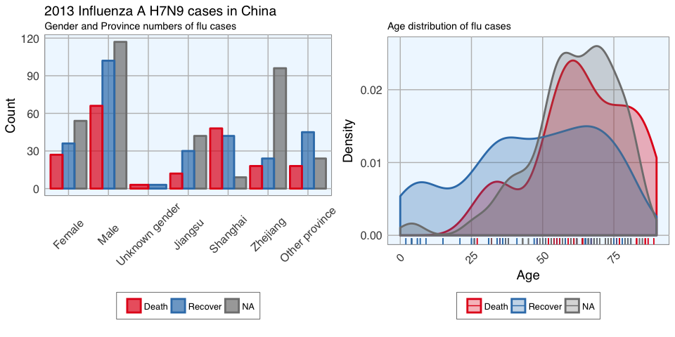
In the dataset, there are more male than female cases and correspondingly, we see more deaths, recoveries and unknown outcomes in men than in women. This is potentially a problem later on for modeling because the inherent likelihoods for outcome are not directly comparable between the sexes.
Most unknown outcomes were recorded in Zhejiang. Similarly to gender, we don’t have an equal distribution of data points across provinces either.
When we look at the age distribution it is obvious that people who died tended to be slightly older than those who recovered. The density curve of unknown outcomes is more similar to that of death than of recovery, suggesting that among these people there might have been more deaths than recoveries.
And lastly, I want to plot how many days passed between onset, hospitalisation and outcome for each case.
ggplot(data = fluH7N9.china.2013_gather, aes(x = Date, y = age, color = outcome)) +
  geom_point(aes(shape = gender), size = 1.5, alpha = 0.6) +
  geom_path(aes(group = case.ID)) +
  facet_wrap( ~ province, ncol = 2) +
  my_theme() +
  scale_shape_manual(values = c(15, 16, 17)) +
  scale_color_brewer(palette="Set1", na.value = "grey50") +
  scale_fill_brewer(palette="Set1") +
  labs(
    color = "Outcome",
    shape = "Gender",
    x = "Date in 2013",
    y = "Age",
    title = "2013 Influenza A H7N9 cases in China",
    subtitle = "Dataset from 'outbreaks' package (Kucharski et al. 2014)",
    caption = "\nTime from onset of flu to outcome."
  )
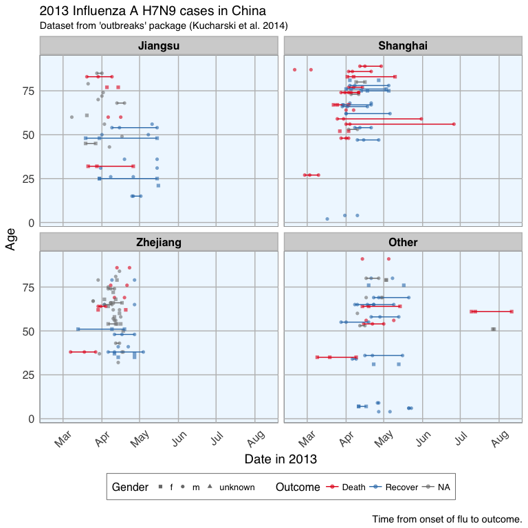
This plot shows that there are many missing values in the dates, so it is hard to draw a general conclusion.
Features
In Machine Learning-speak features are the variables used for model training. Using the right features dramatically influences the accuracy of the model.
Because we don’t have many features, I am keeping age as it is, but I am also generating new features:
- from the date information I am calculating the days between onset and outcome and between onset and hospitalisation
- I am converting gender into numeric values with 1 for female and 0 for male
- similarly, I am converting provinces to binary classifiers (yes == 1, no == 0) for Shanghai, Zhejiang, Jiangsu and other provinces
- the same binary classification is given for whether a case was hospitalised, and whether they had an early onset or early outcome (earlier than the median date)
# preparing the data frame for modeling
#
library(dplyr)

dataset <- fluH7N9.china.2013 %>%
  mutate(hospital = as.factor(ifelse(is.na(date.of.hospitalisation), 0, 1)),
         gender_f = as.factor(ifelse(gender == "f", 1, 0)),
         province_Jiangsu = as.factor(ifelse(province == "Jiangsu", 1, 0)),
         province_Shanghai = as.factor(ifelse(province == "Shanghai", 1, 0)),
         province_Zhejiang = as.factor(ifelse(province == "Zhejiang", 1, 0)),
         province_other = as.factor(ifelse(province == "Zhejiang" | province == "Jiangsu" | province == "Shanghai", 0, 1)),
         days_onset_to_outcome = as.numeric(as.character(gsub(" days", "",
                                      as.Date(as.character(date.of.outcome), format = "%Y-%m-%d") -
                                        as.Date(as.character(date.of.onset), format = "%Y-%m-%d")))),
         days_onset_to_hospital = as.numeric(as.character(gsub(" days", "",
                                      as.Date(as.character(date.of.hospitalisation), format = "%Y-%m-%d") -
                                        as.Date(as.character(date.of.onset), format = "%Y-%m-%d")))),
         age = as.numeric(as.character(age)),
         early_onset = as.factor(ifelse(date.of.onset < summary(fluH7N9.china.2013$date.of.onset)[[3]], 1, 0)),
         early_outcome = as.factor(ifelse(date.of.outcome < summary(fluH7N9.china.2013$date.of.outcome)[[3]], 1, 0))) %>%
  subset(select = -c(2:4, 6, 8))
rownames(dataset) <- dataset$case.ID
dataset <- dataset[, -1]
head(dataset)
##        outcome age hospital gender_f province_Jiangsu province_Shanghai province_Zhejiang province_other days_onset_to_outcome days_onset_to_hospital early_onset early_outcome
## case_1   Death  87        0        0                0                 1                 0              0                    13                     NA           1             1
## case_2   Death  27        1        0                0                 1                 0              0                    11                      4           1             1
## case_3   Death  35        1        1                0                 0                 0              1                    31                     10           1             1
## case_4    <NA>  45        1        1                1                 0                 0              0                    NA                      8           1          <NA>
## case_5 Recover  48        1        1                1                 0                 0              0                    57                     11           1             0
## case_6   Death  32        1        1                1                 0                 0              0                    36                      7           1             1
Imputing missing values
When looking at the dataset I created for modeling, it is obvious that we have quite a few missing values.
The missing values from the outcome column are what I want to predict but for the rest I would either have to remove the entire row from the data or impute the missing information. I decided to try the latter with the mice package.
# impute missing data

library(mice)

dataset_impute <- mice(dataset[, -1],  print = FALSE)
dataset_impute
## Multiply imputed dataset
## Call:
## mice(data = dataset[, -1], printFlag = FALSE)
## Number of multiple imputations:  5
## Missing cells per column:
##                    age               hospital               gender_f       province_Jiangsu      province_Shanghai      province_Zhejiang         province_other  days_onset_to_outcome days_onset_to_hospital            early_onset          early_outcome
##                      2                      0                      2                      0                      0                      0                      0                     67                     74                     10                     65
## Imputation methods:
##                    age               hospital               gender_f       province_Jiangsu      province_Shanghai      province_Zhejiang         province_other  days_onset_to_outcome days_onset_to_hospital            early_onset          early_outcome
##                  "pmm"                     ""               "logreg"                     ""                     ""                     ""                     ""                  "pmm"                  "pmm"               "logreg"               "logreg"
## VisitSequence:
##                    age               gender_f  days_onset_to_outcome days_onset_to_hospital            early_onset          early_outcome
##                      1                      3                      8                      9                     10                     11
## PredictorMatrix:
##                        age hospital gender_f province_Jiangsu province_Shanghai province_Zhejiang province_other days_onset_to_outcome days_onset_to_hospital early_onset early_outcome
## age                      0        1        1                1                 1                 1              1                     1                      1           1             1
## hospital                 0        0        0                0                 0                 0              0                     0                      0           0             0
## gender_f                 1        1        0                1                 1                 1              1                     1                      1           1             1
## province_Jiangsu         0        0        0                0                 0                 0              0                     0                      0           0             0
## province_Shanghai        0        0        0                0                 0                 0              0                     0                      0           0             0
## province_Zhejiang        0        0        0                0                 0                 0              0                     0                      0           0             0
## province_other           0        0        0                0                 0                 0              0                     0                      0           0             0
## days_onset_to_outcome    1        1        1                1                 1                 1              1                     0                      1           1             1
## days_onset_to_hospital   1        1        1                1                 1                 1              1                     1                      0           1             1
## early_onset              1        1        1                1                 1                 1              1                     1                      1           0             1
## early_outcome            1        1        1                1                 1                 1              1                     1                      1           1             0
## Random generator seed value:  NA
# recombine imputed data frame with the outcome column

dataset_complete <- merge(dataset[, 1, drop = FALSE], mice::complete(dataset_impute, 1), by = "row.names", all = TRUE)
rownames(dataset_complete) <- dataset_complete$Row.names
dataset_complete <- dataset_complete[, -1]
Test, train and validation datasets
For building the model, I am separating the imputed data frame into training and test data. Test data are the 57 cases with unknown outcome.
summary(dataset$outcome)
##   Death Recover    NA's
##      32      47      57
The training data will be further devided for validation of the models: 70% of the training data will be kept for model building and the remaining 30% will be used for model testing.
I am using the caret package for modeling.
train_index <- which(is.na(dataset_complete$outcome))
train_data <- dataset_complete[-train_index, ]
test_data  <- dataset_complete[train_index, -1]

library(caret)
set.seed(27)
val_index <- createDataPartition(train_data$outcome, p = 0.7, list=FALSE)
val_train_data <- train_data[val_index, ]
val_test_data  <- train_data[-val_index, ]
val_train_X <- val_train_data[,-1]
val_test_X <- val_test_data[,-1]
Decision trees
To get an idea about how each feature contributes to the prediction of the outcome, I first built a decision tree based on the training data using rpart and rattle.
library(rpart)
library(rattle)
library(rpart.plot)
library(RColorBrewer)

set.seed(27)
fit <- rpart(outcome ~ .,
                    data = train_data,
                    method = "class",
                    control = rpart.control(xval = 10, minbucket = 2, cp = 0), parms = list(split = "information"))

fancyRpartPlot(fit)
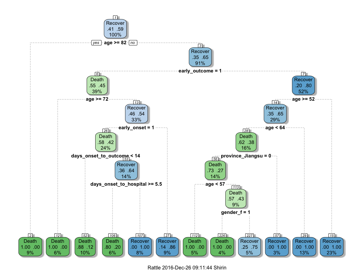
This randomly generated decision tree shows that cases with an early outcome were most likely to die when they were 68 or older, when they also had an early onset and when they were sick for fewer than 13 days. If a person was not among the first cases and was younger than 52, they had a good chance of recovering, but if they were 82 or older, they were more likely to die from the flu.
Feature Importance
Not all of the features I created will be equally important to the model. The decision tree already gave me an idea of which features might be most important but I also want to estimate feature importance using a Random Forest approach with repeated cross validation.
# prepare training scheme
control <- trainControl(method = "repeatedcv", number = 10, repeats = 10)

# train the model
set.seed(27)
model <- train(outcome ~ ., data = train_data, method = "rf", preProcess = NULL, trControl = control)

# estimate variable importance
importance <- varImp(model, scale=TRUE)
# prepare for plotting
importance_df_1 <- importance$importance
importance_df_1$group <- rownames(importance_df_1)

importance_df_1$group <- mapvalues(importance_df_1$group,
                                           from = c("age", "hospital2", "gender_f2", "province_Jiangsu2", "province_Shanghai2", "province_Zhejiang2",
                                                    "province_other2", "days_onset_to_outcome", "days_onset_to_hospital", "early_onset2", "early_outcome2" ),
                                           to = c("Age", "Hospital", "Female", "Jiangsu", "Shanghai", "Zhejiang",
                                                    "Other province", "Days onset to outcome", "Days onset to hospital", "Early onset", "Early outcome" ))
f = importance_df_1[order(importance_df_1$Overall, decreasing = FALSE), "group"]

importance_df_2 <- importance_df_1
importance_df_2$Overall <- 0

importance_df <- rbind(importance_df_1, importance_df_2)

# setting factor levels
importance_df <- within(importance_df, group <- factor(group, levels = f))
importance_df_1 <- within(importance_df_1, group <- factor(group, levels = f))

ggplot() +
  geom_point(data = importance_df_1, aes(x = Overall, y = group, color = group), size = 2) +
  geom_path(data = importance_df, aes(x = Overall, y = group, color = group, group = group), size = 1) +
  scale_color_manual(values = rep(brewer.pal(1, "Set1")[1], 11)) +
  my_theme() +
  theme(legend.position = "none",
        axis.text.x = element_text(angle = 0, vjust = 0.5, hjust = 0.5)) +
  labs(
    x = "Importance",
    y = "",
    title = "2013 Influenza A H7N9 cases in China",
    subtitle = "Scaled feature importance",
    caption = "\nDetermined with Random Forest and
    repeated cross validation (10 repeats, 10 times)"
  )
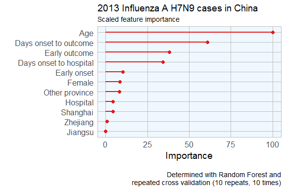
This tells me that age is the most important determining factor for predicting disease outcome, followed by days between onset an outcome, early outcome and days between onset and hospitalisation.
Feature Plot
Before I start actually building models, I want to check whether the distribution of feature values is comparable between training, validation and test datasets.
# prepare for plotting
dataset_complete_gather <- dataset_complete %>%
  mutate(set = ifelse(rownames(dataset_complete) %in% rownames(test_data), "Test Data",
                               ifelse(rownames(dataset_complete) %in% rownames(val_train_data), "Validation Train Data",
                                      ifelse(rownames(dataset_complete) %in% rownames(val_test_data), "Validation Test Data", "NA"))),
         case_ID = rownames(.)) %>%
  gather(group, value, age:early_outcome)

dataset_complete_gather$group <- mapvalues(dataset_complete_gather$group,
                                           from = c("age", "hospital", "gender_f", "province_Jiangsu", "province_Shanghai", "province_Zhejiang",
                                                    "province_other", "days_onset_to_outcome", "days_onset_to_hospital", "early_onset", "early_outcome" ),
                                           to = c("Age", "Hospital", "Female", "Jiangsu", "Shanghai", "Zhejiang",
                                                    "Other province", "Days onset to outcome", "Days onset to hospital", "Early onset", "Early outcome" ))
ggplot(data = dataset_complete_gather, aes(x = as.numeric(value), fill = outcome, color = outcome)) +
  geom_density(alpha = 0.2) +
  geom_rug() +
  scale_color_brewer(palette="Set1", na.value = "grey50") +
  scale_fill_brewer(palette="Set1", na.value = "grey50") +
  my_theme() +
  facet_wrap(set ~ group, ncol = 11, scales = "free") +
  labs(
    x = "Value",
    y = "Density",
    title = "2013 Influenza A H7N9 cases in China",
    subtitle = "Features for classifying outcome",
    caption = "\nDensity distribution of all features used for classification of flu outcome."
  )
ggplot(subset(dataset_complete_gather, group == "Age" | group == "Days onset to hospital" | group == "Days onset to outcome"),
       aes(x=outcome, y=as.numeric(value), fill=set)) + geom_boxplot() +
  my_theme() +
  scale_fill_brewer(palette="Set1", type = "div ") +
  facet_wrap( ~ group, ncol = 3, scales = "free") +
  labs(
    fill = "",
    x = "Outcome",
    y = "Value",
    title = "2013 Influenza A H7N9 cases in China",
    subtitle = "Features for classifying outcome",
    caption = "\nBoxplot of the features age, days from onset to hospitalisation and days from onset to outcome."
  )
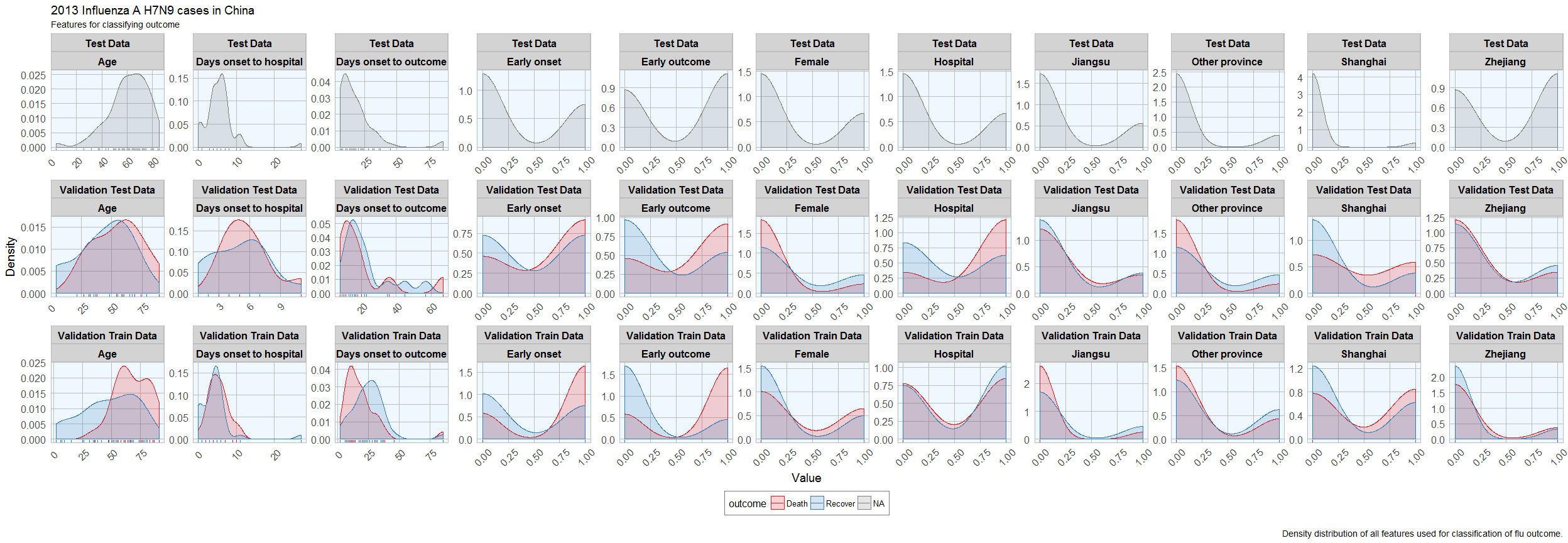
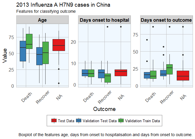
Luckily, the distributions looks reasonably similar between the validation and test data, except for a few outliers.
Comparing Machine Learning algorithms
Before I try to predict the outcome of the unknown cases, I am testing the models’ accuracy with the validation datasets on a couple of algorithms. I have chosen only a few more well known algorithms, but caret implements many more.
I have chose to not do any preprocessing because I was worried that the different data distributions with continuous variables (e.g. age) and binary variables (i.e. 0, 1 classification of e.g. hospitalisation) would lead to problems.
Random Forest
Random Forests predictions are based on the generation of multiple classification trees.
This model classified 14 out of 23 cases correctly.
set.seed(27)
model_rf <- caret::train(outcome ~ .,
                             data = val_train_data,
                             method = "rf",
                             preProcess = NULL,
                             trControl = trainControl(method = "repeatedcv", number = 10, repeats = 10, verboseIter = FALSE))
model_rf
## Random Forest
##
## 56 samples
## 11 predictors
##  2 classes: 'Death', 'Recover'
##
## No pre-processing
## Resampling: Cross-Validated (10 fold, repeated 10 times)
## Summary of sample sizes: 50, 50, 51, 51, 51, 50, ...
## Resampling results across tuning parameters:
##
##   mtry  Accuracy   Kappa
##    2    0.7801905  0.5338408
##    6    0.7650952  0.4926366
##   11    0.7527619  0.4638073
##
## Accuracy was used to select the optimal model using  the largest value.
## The final value used for the model was mtry = 2.
confusionMatrix(predict(model_rf, val_test_data[, -1]), val_test_data$outcome)
## Confusion Matrix and Statistics
##
##           Reference
## Prediction Death Recover
##    Death       4       4
##    Recover     5      10
##
##                Accuracy : 0.6087
##                  95% CI : (0.3854, 0.8029)
##     No Information Rate : 0.6087
##     P-Value [Acc > NIR] : 0.5901
##
##                   Kappa : 0.1619
##  Mcnemar's Test P-Value : 1.0000
##
##             Sensitivity : 0.4444
##             Specificity : 0.7143
##          Pos Pred Value : 0.5000
##          Neg Pred Value : 0.6667
##              Prevalence : 0.3913
##          Detection Rate : 0.1739
##    Detection Prevalence : 0.3478
##       Balanced Accuracy : 0.5794
##
##        'Positive' Class : Death
##
Elastic-Net Regularized Generalized Linear Models
Lasso or elastic net regularization for generalized linear model regression are based on linear regression models and is useful when we have feature correlation in our model.
This model classified 13 out of 23 cases correctly.
set.seed(27)
model_glmnet <- caret::train(outcome ~ .,
                             data = val_train_data,
                             method = "glmnet",
                             preProcess = NULL,
                             trControl = trainControl(method = "repeatedcv", number = 10, repeats = 10, verboseIter = FALSE))
model_glmnet
## glmnet
##
## 56 samples
## 11 predictors
##  2 classes: 'Death', 'Recover'
##
## No pre-processing
## Resampling: Cross-Validated (10 fold, repeated 10 times)
## Summary of sample sizes: 50, 50, 51, 51, 51, 50, ...
## Resampling results across tuning parameters:
##
##   alpha  lambda        Accuracy   Kappa
##   0.10   0.0005154913  0.7211905  0.4218952
##   0.10   0.0051549131  0.7189524  0.4189835
##   0.10   0.0515491312  0.7469524  0.4704687
##   0.55   0.0005154913  0.7211905  0.4218952
##   0.55   0.0051549131  0.7236190  0.4280528
##   0.55   0.0515491312  0.7531905  0.4801031
##   1.00   0.0005154913  0.7228571  0.4245618
##   1.00   0.0051549131  0.7278571  0.4361809
##   1.00   0.0515491312  0.7678571  0.5094194
##
## Accuracy was used to select the optimal model using  the largest value.
## The final values used for the model were alpha = 1 and lambda = 0.05154913.
confusionMatrix(predict(model_glmnet, val_test_data[, -1]), val_test_data$outcome)
## Confusion Matrix and Statistics
##
##           Reference
## Prediction Death Recover
##    Death       3       4
##    Recover     6      10
##
##                Accuracy : 0.5652
##                  95% CI : (0.3449, 0.7681)
##     No Information Rate : 0.6087
##     P-Value [Acc > NIR] : 0.7418
##
##                   Kappa : 0.0496
##  Mcnemar's Test P-Value : 0.7518
##
##             Sensitivity : 0.3333
##             Specificity : 0.7143
##          Pos Pred Value : 0.4286
##          Neg Pred Value : 0.6250
##              Prevalence : 0.3913
##          Detection Rate : 0.1304
##    Detection Prevalence : 0.3043
##       Balanced Accuracy : 0.5238
##
##        'Positive' Class : Death
##
k-Nearest Neighbors
k-nearest neighbors predicts based on point distances with predefined constants.
This model classified 14 out of 23 cases correctly.
set.seed(27)
model_kknn <- caret::train(outcome ~ .,
                             data = val_train_data,
                             method = "kknn",
                             preProcess = NULL,
                             trControl = trainControl(method = "repeatedcv", number = 10, repeats = 10, verboseIter = FALSE))
model_kknn
## k-Nearest Neighbors
##
## 56 samples
## 11 predictors
##  2 classes: 'Death', 'Recover'
##
## No pre-processing
## Resampling: Cross-Validated (10 fold, repeated 10 times)
## Summary of sample sizes: 50, 50, 51, 51, 51, 50, ...
## Resampling results across tuning parameters:
##
##   kmax  Accuracy   Kappa
##   5     0.6531905  0.2670442
##   7     0.7120476  0.4031836
##   9     0.7106190  0.4004564
##
## Tuning parameter 'distance' was held constant at a value of 2
## Tuning parameter 'kernel' was held constant at a value of optimal
## Accuracy was used to select the optimal model using  the largest value.
## The final values used for the model were kmax = 7, distance = 2 and kernel = optimal.
confusionMatrix(predict(model_kknn, val_test_data[, -1]), val_test_data$outcome)
## Confusion Matrix and Statistics
##
##           Reference
## Prediction Death Recover
##    Death       3       3
##    Recover     6      11
##
##                Accuracy : 0.6087
##                  95% CI : (0.3854, 0.8029)
##     No Information Rate : 0.6087
##     P-Value [Acc > NIR] : 0.5901
##
##                   Kappa : 0.1266
##  Mcnemar's Test P-Value : 0.5050
##
##             Sensitivity : 0.3333
##             Specificity : 0.7857
##          Pos Pred Value : 0.5000
##          Neg Pred Value : 0.6471
##              Prevalence : 0.3913
##          Detection Rate : 0.1304
##    Detection Prevalence : 0.2609
##       Balanced Accuracy : 0.5595
##
##        'Positive' Class : Death
##
Penalized Discriminant Analysis
Penalized Discriminant Analysis is the penalized linear discriminant analysis and is also useful for when we have highly correlated features.
This model classified 14 out of 23 cases correctly.
set.seed(27)
model_pda <- caret::train(outcome ~ .,
                             data = val_train_data,
                             method = "pda",
                             preProcess = NULL,
                             trControl = trainControl(method = "repeatedcv", number = 10, repeats = 10, verboseIter = FALSE))
model_pda
## Penalized Discriminant Analysis
##
## 56 samples
## 11 predictors
##  2 classes: 'Death', 'Recover'
##
## No pre-processing
## Resampling: Cross-Validated (10 fold, repeated 10 times)
## Summary of sample sizes: 50, 50, 51, 51, 51, 50, ...
## Resampling results across tuning parameters:
##
##   lambda  Accuracy   Kappa
##   0e+00         NaN        NaN
##   1e-04   0.7255238  0.4373766
##   1e-01   0.7235238  0.4342554
##
## Accuracy was used to select the optimal model using  the largest value.
## The final value used for the model was lambda = 1e-04.
confusionMatrix(predict(model_pda, val_test_data[, -1]), val_test_data$outcome)
## Confusion Matrix and Statistics
##
##           Reference
## Prediction Death Recover
##    Death       4       4
##    Recover     5      10
##
##                Accuracy : 0.6087
##                  95% CI : (0.3854, 0.8029)
##     No Information Rate : 0.6087
##     P-Value [Acc > NIR] : 0.5901
##
##                   Kappa : 0.1619
##  Mcnemar's Test P-Value : 1.0000
##
##             Sensitivity : 0.4444
##             Specificity : 0.7143
##          Pos Pred Value : 0.5000
##          Neg Pred Value : 0.6667
##              Prevalence : 0.3913
##          Detection Rate : 0.1739
##    Detection Prevalence : 0.3478
##       Balanced Accuracy : 0.5794
##
##        'Positive' Class : Death
##
Stabilized Linear Discriminant Analysis
Stabilized Linear Discriminant Analysis is designed for high-dimensional data and correlated co-variables.
This model classified 15 out of 23 cases correctly.
set.seed(27)
model_slda <- caret::train(outcome ~ .,
                             data = val_train_data,
                             method = "slda",
                             preProcess = NULL,
                             trControl = trainControl(method = "repeatedcv", number = 10, repeats = 10, verboseIter = FALSE))
model_slda
## Stabilized Linear Discriminant Analysis
##
## 56 samples
## 11 predictors
##  2 classes: 'Death', 'Recover'
##
## No pre-processing
## Resampling: Cross-Validated (10 fold, repeated 10 times)
## Summary of sample sizes: 50, 50, 51, 51, 51, 50, ...
## Resampling results:
##
##   Accuracy   Kappa
##   0.6886667  0.3512234
##
##
confusionMatrix(predict(model_slda, val_test_data[, -1]), val_test_data$outcome)
## Confusion Matrix and Statistics
##
##           Reference
## Prediction Death Recover
##    Death       3       2
##    Recover     6      12
##
##                Accuracy : 0.6522
##                  95% CI : (0.4273, 0.8362)
##     No Information Rate : 0.6087
##     P-Value [Acc > NIR] : 0.4216
##
##                   Kappa : 0.2069
##  Mcnemar's Test P-Value : 0.2888
##
##             Sensitivity : 0.3333
##             Specificity : 0.8571
##          Pos Pred Value : 0.6000
##          Neg Pred Value : 0.6667
##              Prevalence : 0.3913
##          Detection Rate : 0.1304
##    Detection Prevalence : 0.2174
##       Balanced Accuracy : 0.5952
##
##        'Positive' Class : Death
##
Nearest Shrunken Centroids
Nearest Shrunken Centroids computes a standardized centroid for each class and shrinks each centroid toward the overall centroid for all classes.
This model classified 15 out of 23 cases correctly.
set.seed(27)
model_pam <- caret::train(outcome ~ .,
                             data = val_train_data,
                             method = "pam",
                             preProcess = NULL,
                             trControl = trainControl(method = "repeatedcv", number = 10, repeats = 10, verboseIter = FALSE))
model_pam
## Nearest Shrunken Centroids
##
## 56 samples
## 11 predictors
##  2 classes: 'Death', 'Recover'
##
## No pre-processing
## Resampling: Cross-Validated (10 fold, repeated 10 times)
## Summary of sample sizes: 50, 50, 51, 51, 51, 50, ...
## Resampling results across tuning parameters:
##
##   threshold  Accuracy   Kappa
##   0.1200215  0.7283333  0.4418904
##   1.7403111  0.6455714  0.2319674
##   3.3606007  0.5904762  0.0000000
##
## Accuracy was used to select the optimal model using  the largest value.
## The final value used for the model was threshold = 0.1200215.
confusionMatrix(predict(model_pam, val_test_data[, -1]), val_test_data$outcome)
## Confusion Matrix and Statistics
##
##           Reference
## Prediction Death Recover
##    Death       4       3
##    Recover     5      11
##
##                Accuracy : 0.6522
##                  95% CI : (0.4273, 0.8362)
##     No Information Rate : 0.6087
##     P-Value [Acc > NIR] : 0.4216
##
##                   Kappa : 0.2397
##  Mcnemar's Test P-Value : 0.7237
##
##             Sensitivity : 0.4444
##             Specificity : 0.7857
##          Pos Pred Value : 0.5714
##          Neg Pred Value : 0.6875
##              Prevalence : 0.3913
##          Detection Rate : 0.1739
##    Detection Prevalence : 0.3043
##       Balanced Accuracy : 0.6151
##
##        'Positive' Class : Death
##
Single C5.0 Tree
C5.0 is another tree-based modeling algorithm.
This model classified 15 out of 23 cases correctly.
set.seed(27)
model_C5.0Tree <- caret::train(outcome ~ .,
                             data = val_train_data,
                             method = "C5.0Tree",
                             preProcess = NULL,
                             trControl = trainControl(method = "repeatedcv", number = 10, repeats = 10, verboseIter = FALSE))
model_C5.0Tree
## Single C5.0 Tree
##
## 56 samples
## 11 predictors
##  2 classes: 'Death', 'Recover'
##
## No pre-processing
## Resampling: Cross-Validated (10 fold, repeated 10 times)
## Summary of sample sizes: 50, 50, 51, 51, 51, 50, ...
## Resampling results:
##
##   Accuracy   Kappa
##   0.7103333  0.4047334
##
##
confusionMatrix(predict(model_C5.0Tree, val_test_data[, -1]), val_test_data$outcome)
## Confusion Matrix and Statistics
##
##           Reference
## Prediction Death Recover
##    Death       5       4
##    Recover     4      10
##
##                Accuracy : 0.6522
##                  95% CI : (0.4273, 0.8362)
##     No Information Rate : 0.6087
##     P-Value [Acc > NIR] : 0.4216
##
##                   Kappa : 0.2698
##  Mcnemar's Test P-Value : 1.0000
##
##             Sensitivity : 0.5556
##             Specificity : 0.7143
##          Pos Pred Value : 0.5556
##          Neg Pred Value : 0.7143
##              Prevalence : 0.3913
##          Detection Rate : 0.2174
##    Detection Prevalence : 0.3913
##       Balanced Accuracy : 0.6349
##
##        'Positive' Class : Death
##
Partial Least Squares
Partial least squares regression combined principal component analysis and multiple regression and is useful for modeling with correlated features.
This model classified 15 out of 23 cases correctly.
set.seed(27)
model_pls <- caret::train(outcome ~ .,
                             data = val_train_data,
                             method = "pls",
                             preProcess = NULL,
                             trControl = trainControl(method = "repeatedcv", number = 10, repeats = 10, verboseIter = FALSE))
model_pls
## Partial Least Squares
##
## 56 samples
## 11 predictors
##  2 classes: 'Death', 'Recover'
##
## No pre-processing
## Resampling: Cross-Validated (10 fold, repeated 10 times)
## Summary of sample sizes: 50, 50, 51, 51, 51, 50, ...
## Resampling results across tuning parameters:
##
##   ncomp  Accuracy   Kappa
##   1      0.6198571  0.2112982
##   2      0.6376190  0.2436222
##   3      0.6773810  0.3305780
##
## Accuracy was used to select the optimal model using  the largest value.
## The final value used for the model was ncomp = 3.
confusionMatrix(predict(model_pls, val_test_data[, -1]), val_test_data$outcome)
## Confusion Matrix and Statistics
##
##           Reference
## Prediction Death Recover
##    Death       3       2
##    Recover     6      12
##
##                Accuracy : 0.6522
##                  95% CI : (0.4273, 0.8362)
##     No Information Rate : 0.6087
##     P-Value [Acc > NIR] : 0.4216
##
##                   Kappa : 0.2069
##  Mcnemar's Test P-Value : 0.2888
##
##             Sensitivity : 0.3333
##             Specificity : 0.8571
##          Pos Pred Value : 0.6000
##          Neg Pred Value : 0.6667
##              Prevalence : 0.3913
##          Detection Rate : 0.1304
##    Detection Prevalence : 0.2174
##       Balanced Accuracy : 0.5952
##
##        'Positive' Class : Death
##
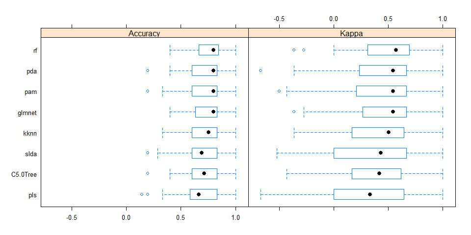
Comparing accuracy of models
All models were similarly accurate.
# Create a list of models
models <- list(rf = model_rf, glmnet = model_glmnet, kknn = model_kknn, pda = model_pda, slda = model_slda,
               pam = model_pam, C5.0Tree = model_C5.0Tree, pls = model_pls)

# Resample the models
resample_results <- resamples(models)

# Generate a summary
summary(resample_results, metric = c("Kappa", "Accuracy"))
##
## Call:
## summary.resamples(object = resample_results, metric = c("Kappa", "Accuracy"))
##
## Models: rf, glmnet, kknn, pda, slda, pam, C5.0Tree, pls
## Number of resamples: 100
##
## Kappa
##             Min. 1st Qu. Median   Mean 3rd Qu. Max. NA's
## rf       -0.3636  0.3214 0.5714 0.5338  0.6800    1    0
## glmnet   -0.3636  0.2768 0.5455 0.5094  0.6667    1    0
## kknn     -0.3636  0.1667 0.5035 0.4032  0.6282    1    0
## pda      -0.6667  0.2431 0.5455 0.4374  0.6667    1    0
## slda     -0.5217  0.0000 0.4308 0.3512  0.6667    1    0
## pam      -0.5000  0.2292 0.5455 0.4419  0.6667    1    0
## C5.0Tree -0.4286  0.1667 0.4167 0.4047  0.6154    1    0
## pls      -0.6667  0.0000 0.3333 0.3306  0.6282    1    0
##
## Accuracy
##            Min. 1st Qu. Median   Mean 3rd Qu. Max. NA's
## rf       0.4000  0.6667 0.8000 0.7802  0.8393    1    0
## glmnet   0.4000  0.6500 0.8000 0.7679  0.8333    1    0
## kknn     0.3333  0.6000 0.7571 0.7120  0.8333    1    0
## pda      0.2000  0.6000 0.8000 0.7255  0.8333    1    0
## slda     0.2000  0.6000 0.6905 0.6887  0.8333    1    0
## pam      0.2000  0.6000 0.8000 0.7283  0.8333    1    0
## C5.0Tree 0.2000  0.6000 0.7143 0.7103  0.8333    1    0
## pls      0.1429  0.5929 0.6667 0.6774  0.8333    1    0
bwplot(resample_results , metric = c("Kappa","Accuracy"))
Combined results of predicting validation test samples
To compare the predictions from all models, I summed up the prediction probabilities for Death and Recovery from all models and calculated the log2 of the ratio between the summed probabilities for Recovery by the summed probabilities for Death. All cases with a log2 ratio bigger than 1.5 were defined as Recover, cases with a log2 ratio below -1.5 were defined as Death, and the remaining cases were defined as uncertain.
results <- data.frame(randomForest = predict(model_rf, newdata = val_test_data[, -1], type="prob"),
                      glmnet = predict(model_glmnet, newdata = val_test_data[, -1], type="prob"),
                      kknn = predict(model_kknn, newdata = val_test_data[, -1], type="prob"),
                      pda = predict(model_pda, newdata = val_test_data[, -1], type="prob"),
                      slda = predict(model_slda, newdata = val_test_data[, -1], type="prob"),
                      pam = predict(model_pam, newdata = val_test_data[, -1], type="prob"),
                      C5.0Tree = predict(model_C5.0Tree, newdata = val_test_data[, -1], type="prob"),
                      pls = predict(model_pls, newdata = val_test_data[, -1], type="prob"))

results$sum_Death <- rowSums(results[, grep("Death", colnames(results))])
results$sum_Recover <- rowSums(results[, grep("Recover", colnames(results))])
results$log2_ratio <- log2(results$sum_Recover/results$sum_Death)
results$true_outcome <- val_test_data$outcome
results$pred_outcome <- ifelse(results$log2_ratio > 1.5, "Recover", ifelse(results$log2_ratio < -1.5, "Death", "uncertain"))
results$prediction <- ifelse(results$pred_outcome == results$true_outcome, "CORRECT",
                             ifelse(results$pred_outcome == "uncertain", "uncertain", "wrong"))
results[, -c(1:16)]
##          sum_Death sum_Recover  log2_ratio true_outcome pred_outcome prediction
## case_123 2.2236374    5.776363  1.37723972        Death    uncertain  uncertain
## case_127 0.7522674    7.247733  3.26821230      Recover      Recover    CORRECT
## case_128 2.4448101    5.555190  1.18411381      Recover    uncertain  uncertain
## case_14  2.9135620    5.086438  0.80387172      Recover    uncertain  uncertain
## case_19  2.2113377    5.788662  1.38831062        Death    uncertain  uncertain
## case_2   3.6899508    4.310049  0.22410277        Death    uncertain  uncertain
## case_20  4.5621189    3.437881 -0.40818442      Recover    uncertain  uncertain
## case_21  4.9960238    3.003976 -0.73390698      Recover    uncertain  uncertain
## case_34  6.1430233    1.856977 -1.72599312        Death        Death    CORRECT
## case_37  0.8717595    7.128241  3.03154401      Recover      Recover    CORRECT
## case_5   1.7574945    6.242505  1.82860496      Recover      Recover    CORRECT
## case_51  3.8917736    4.108226  0.07808791      Recover    uncertain  uncertain
## case_55  3.1548368    4.845163  0.61897986      Recover    uncertain  uncertain
## case_6   3.5163388    4.483661  0.35060317        Death    uncertain  uncertain
## case_61  5.0803241    2.919676 -0.79911232        Death    uncertain  uncertain
## case_65  1.1282313    6.871769  2.60661863      Recover      Recover    CORRECT
## case_74  5.3438427    2.656157 -1.00853699      Recover    uncertain  uncertain
## case_78  3.2183947    4.781605  0.57115378        Death    uncertain  uncertain
## case_79  1.9521617    6.047838  1.63134700      Recover      Recover    CORRECT
## case_8   3.6106045    4.389395  0.28178184        Death    uncertain  uncertain
## case_87  4.9712879    3.028712 -0.71491522        Death    uncertain  uncertain
## case_91  1.8648837    6.135116  1.71800508      Recover      Recover    CORRECT
## case_94  2.1198087    5.880191  1.47192901      Recover    uncertain  uncertain
All predictions based on all models were either correct or uncertain.
Predicting unknown outcomes
The above models will now be used to predict the outcome of cases with unknown fate.
set.seed(27)
model_rf <- caret::train(outcome ~ .,
                             data = train_data,
                             method = "rf",
                             preProcess = NULL,
                             trControl = trainControl(method = "repeatedcv", number = 10, repeats = 10, verboseIter = FALSE))
model_glmnet <- caret::train(outcome ~ .,
                             data = train_data,
                             method = "glmnet",
                             preProcess = NULL,
                             trControl = trainControl(method = "repeatedcv", number = 10, repeats = 10, verboseIter = FALSE))
model_kknn <- caret::train(outcome ~ .,
                             data = train_data,
                             method = "kknn",
                             preProcess = NULL,
                             trControl = trainControl(method = "repeatedcv", number = 10, repeats = 10, verboseIter = FALSE))
model_pda <- caret::train(outcome ~ .,
                             data = train_data,
                             method = "pda",
                             preProcess = NULL,
                             trControl = trainControl(method = "repeatedcv", number = 10, repeats = 10, verboseIter = FALSE))
model_slda <- caret::train(outcome ~ .,
                             data = train_data,
                             method = "slda",
                             preProcess = NULL,
                             trControl = trainControl(method = "repeatedcv", number = 10, repeats = 10, verboseIter = FALSE))
model_pam <- caret::train(outcome ~ .,
                             data = train_data,
                             method = "pam",
                             preProcess = NULL,
                             trControl = trainControl(method = "repeatedcv", number = 10, repeats = 10, verboseIter = FALSE))
model_C5.0Tree <- caret::train(outcome ~ .,
                             data = train_data,
                             method = "C5.0Tree",
                             preProcess = NULL,
                             trControl = trainControl(method = "repeatedcv", number = 10, repeats = 10, verboseIter = FALSE))
model_pls <- caret::train(outcome ~ .,
                             data = train_data,
                             method = "pls",
                             preProcess = NULL,
                             trControl = trainControl(method = "repeatedcv", number = 10, repeats = 10, verboseIter = FALSE))

models <- list(rf = model_rf, glmnet = model_glmnet, kknn = model_kknn, pda = model_pda, slda = model_slda,
               pam = model_pam, C5.0Tree = model_C5.0Tree, pls = model_pls)

# Resample the models
resample_results <- resamples(models)

bwplot(resample_results , metric = c("Kappa","Accuracy"))
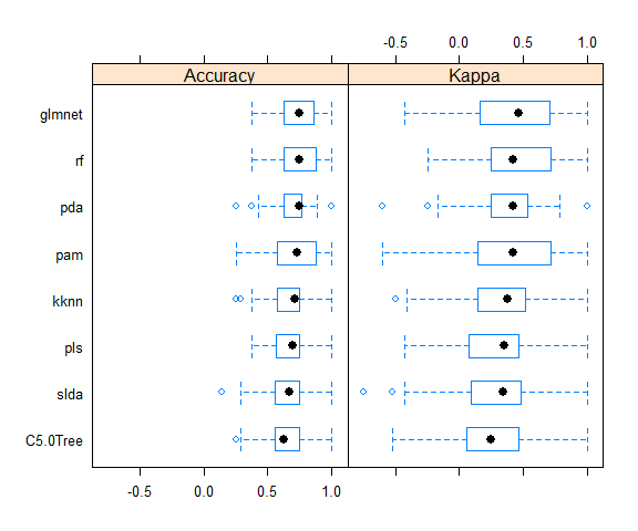
Here again, the accuracy is similar in all models.
The final results are calculate as described above.
results <- data.frame(randomForest = predict(model_rf, newdata = test_data, type="prob"),
                      glmnet = predict(model_glmnet, newdata = test_data, type="prob"),
                      kknn = predict(model_kknn, newdata = test_data, type="prob"),
                      pda = predict(model_pda, newdata = test_data, type="prob"),
                      slda = predict(model_slda, newdata = test_data, type="prob"),
                      pam = predict(model_pam, newdata = test_data, type="prob"),
                      C5.0Tree = predict(model_C5.0Tree, newdata = test_data, type="prob"),
                      pls = predict(model_pls, newdata = test_data, type="prob"))

results$sum_Death <- rowSums(results[, grep("Death", colnames(results))])
results$sum_Recover <- rowSums(results[, grep("Recover", colnames(results))])
results$log2_ratio <- log2(results$sum_Recover/results$sum_Death)
results$predicted_outcome <- ifelse(results$log2_ratio > 1.5, "Recover", ifelse(results$log2_ratio < -1.5, "Death", "uncertain"))
results[, -c(1:16)]
##          sum_Death sum_Recover  log2_ratio predicted_outcome
## case_100 3.6707808    4.329219  0.23801986         uncertain
## case_101 6.3194220    1.680578 -1.91083509             Death
## case_102 6.4960471    1.503953 -2.11080274             Death
## case_103 2.3877223    5.612278  1.23295134         uncertain
## case_104 4.1254604    3.874540 -0.09053024         uncertain
## case_105 2.1082161    5.891784  1.48268174         uncertain
## case_108 6.5941436    1.405856 -2.22973606             Death
## case_109 2.2780779    5.721922  1.32868278         uncertain
## case_110 1.7853361    6.214664  1.79948072           Recover
## case_112 4.5102439    3.489756 -0.37007925         uncertain
## case_113 4.7047554    3.295245 -0.51373420         uncertain
## case_114 1.6397105    6.360290  1.95565132           Recover
## case_115 1.2351519    6.764848  2.45336902           Recover
## case_118 1.4675571    6.532443  2.15420601           Recover
## case_120 1.9322149    6.067785  1.65091447           Recover
## case_122 1.1165786    6.883421  2.62404109           Recover
## case_126 5.4933927    2.506607 -1.13196145         uncertain
## case_130 4.3035732    3.696427 -0.21940367         uncertain
## case_132 5.0166184    2.983382 -0.74976671         uncertain
## case_136 2.6824566    5.317543  0.98720505         uncertain
## case_15  5.8545370    2.145463 -1.44826607         uncertain
## case_16  6.5063794    1.493621 -2.12304122             Death
## case_22  4.2929861    3.707014 -0.21172398         uncertain
## case_28  6.6129447    1.387055 -2.25326754             Death
## case_31  6.2625800    1.737420 -1.84981057             Death
## case_32  6.0986316    1.901368 -1.68144746             Death
## case_38  1.7581540    6.241846  1.82791134           Recover
## case_39  2.4765188    5.523481  1.15726428         uncertain
## case_4   5.1309910    2.869009 -0.83868503         uncertain
## case_40  6.6069297    1.393070 -2.24571191             Death
## case_41  5.5499144    2.450086 -1.17963336         uncertain
## case_42  2.0709160    5.929084  1.51754019           Recover
## case_47  6.1988812    1.801119 -1.78311450             Death
## case_48  5.6500772    2.349923 -1.26565724         uncertain
## case_52  5.9096543    2.090346 -1.49933214         uncertain
## case_54  2.6763066    5.323693  0.99218409         uncertain
## case_56  2.6826414    5.317359  0.98705557         uncertain
## case_62  6.0722552    1.927745 -1.65531833             Death
## case_63  3.9541381    4.045862  0.03308379         uncertain
## case_66  5.8320010    2.167999 -1.42762690         uncertain
## case_67  2.1732059    5.826794  1.42287745         uncertain
## case_68  4.3464174    3.653583 -0.25051491         uncertain
## case_69  1.8902845    6.109715  1.69250181           Recover
## case_70  4.5986242    3.401376 -0.43508393         uncertain
## case_71  2.7966938    5.203306  0.89570626         uncertain
## case_80  2.7270986    5.272901  0.95123017         uncertain
## case_84  1.9485253    6.051475  1.63490411           Recover
## case_85  3.0076953    4.992305  0.73104755         uncertain
## case_86  2.0417802    5.958220  1.54505376           Recover
## case_88  0.7285419    7.271458  3.31916083           Recover
## case_9   2.2188620    5.781138  1.38153353         uncertain
## case_90  1.3973262    6.602674  2.24038155           Recover
## case_92  5.0994993    2.900501 -0.81405366         uncertain
## case_93  4.3979048    3.602095 -0.28798006         uncertain
## case_95  3.5561792    4.443821  0.32147260         uncertain
## case_96  1.3359082    6.664092  2.31858744           Recover
## case_99  5.0776686    2.922331 -0.79704644         uncertain
From 57 cases, 14 were defined as Recover, 10 as Death and 33 as uncertain.
results_combined <- merge(results[, -c(1:16)], fluH7N9.china.2013[which(fluH7N9.china.2013$case.ID %in% rownames(results)), ],
                          by.x = "row.names", by.y = "case.ID")
results_combined <- results_combined[, -c(2, 3, 8, 9)]
results_combined_gather <- results_combined %>%
  gather(group_dates, date, date.of.onset:date.of.hospitalisation)

results_combined_gather$group_dates <- factor(results_combined_gather$group_dates, levels = c("date.of.onset", "date.of.hospitalisation"))

results_combined_gather$group_dates <- mapvalues(results_combined_gather$group_dates, from = c("date.of.onset", "date.of.hospitalisation"),
                                             to = c("Date of onset", "Date of hospitalisation"))

results_combined_gather$gender <- mapvalues(results_combined_gather$gender, from = c("f", "m"),
                                             to = c("Female", "Male"))
levels(results_combined_gather$gender) <- c(levels(results_combined_gather$gender), "unknown")
results_combined_gather$gender[is.na(results_combined_gather$gender)] <- "unknown"
results_combined_gather$age <- as.numeric(as.character(results_combined_gather$age))
ggplot(data = results_combined_gather, aes(x = date, y = log2_ratio, color = predicted_outcome)) +
  geom_jitter(aes(size = age), alpha = 0.3) +
  geom_rug() +
  facet_grid(gender ~ group_dates) +
  labs(
    color = "Predicted outcome",
    size = "Age",
    x = "Date in 2013",
    y = "log2 ratio of prediction Recover vs Death",
    title = "2013 Influenza A H7N9 cases in China",
    subtitle = "Predicted outcome",
    caption = ""
  ) +
  my_theme() +
  scale_color_brewer(palette="Set1") +
  scale_fill_brewer(palette="Set1")
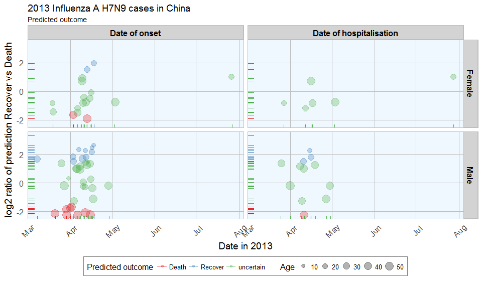
The comparison of date of onset, data of hospitalisation, gender and age with predicted outcome shows that predicted deaths were associated with older age than predicted Recoveries. Date of onset does not show an obvious bias in either direction.
Conclusions
This dataset posed a couple of difficulties to begin with, like unequal distribution of data points across variables and missing data. This makes the modeling inherently prone to flaws. However, real life data isn’t perfect either, so I went ahead and tested the modeling success anyway.
By accounting for uncertain classification with low predictions probability, the validation data could be classified accurately. However, for a more accurate model, these few cases don’t give enough information to reliably predict the outcome. More cases, more information (i.e. more features) and fewer missing data would improve the modeling outcome.
Also, this example is only applicable for this specific case of flu. In order to be able to draw more general conclusions about flu outcome, other cases and additional information, for example on medical parameters like preexisting medical conditions, disase parameters, demographic information, etc. would be necessary.
All in all, this dataset served as a nice example of the possibilities (and pitfalls) of machine learning applications and showcases a basic workflow for building prediction models with R.
For a comparison of feature selection methods see here.
If you see any mistakes or have tips and tricks for improvement, please don’t hesitate to let me know! Thanks. :-)
If you are interested in more machine learning posts, check out the category listing for machine_learning.
sessionInfo()
## R version 3.3.2 (2016-10-31)
## Platform: x86_64-w64-mingw32/x64 (64-bit)
## Running under: Windows 7 x64 (build 7601) Service Pack 1
##
## locale:
## [1] LC_COLLATE=English_United States.1252  LC_CTYPE=English_United States.1252    LC_MONETARY=English_United States.1252 LC_NUMERIC=C                           LC_TIME=English_United States.1252
##
## attached base packages:
## [1] grid      stats     graphics  grDevices utils     datasets  methods   base
##
## other attached packages:
##  [1] pls_2.5-0           C50_0.1.0-24        pamr_1.55           survival_2.40-1     cluster_2.0.5       ipred_0.9-5         mda_0.4-9           class_7.3-14        kknn_1.3.1          glmnet_2.0-5        foreach_1.4.3       Matrix_1.2-7.1      randomForest_4.6-12 RColorBrewer_1.1-2  rpart.plot_2.1.0    rattle_4.1.0        rpart_4.1-10        caret_6.0-73        lattice_0.20-34     mice_2.25           Rcpp_0.12.7         dplyr_0.5.0         gridExtra_2.2.1     ggplot2_2.2.0       plyr_1.8.4          tidyr_0.6.0         outbreaks_1.0.0
##
## loaded via a namespace (and not attached):
##  [1] RGtk2_2.20.31      assertthat_0.1     digest_0.6.10      R6_2.2.0           MatrixModels_0.4-1 stats4_3.3.2       evaluate_0.10      e1071_1.6-7        lazyeval_0.2.0     minqa_1.2.4        SparseM_1.74       car_2.1-3          nloptr_1.0.4       partykit_1.1-1     rmarkdown_1.1      labeling_0.3       splines_3.3.2      lme4_1.1-12        stringr_1.1.0      igraph_1.0.1       munsell_0.4.3      compiler_3.3.2     mgcv_1.8-16        htmltools_0.3.5    nnet_7.3-12        tibble_1.2         prodlim_1.5.7      codetools_0.2-15   MASS_7.3-45        ModelMetrics_1.1.0 nlme_3.1-128       gtable_0.2.0       DBI_0.5-1          magrittr_1.5       scales_0.4.1       stringi_1.1.2      reshape2_1.4.2     Formula_1.2-1      lava_1.4.5         iterators_1.0.8    tools_3.3.2        parallel_3.3.2     pbkrtest_0.4-6     yaml_2.1.14        colorspace_1.3-0   knitr_1.15         quantreg_5.29


